(Study on Agricultural Management for Sustainable Agriculture in Zhangye Oasis, Middle Reaches of Heihe River Basin)

Sustainable Agriculture in Zhangye Oasis, Middle Reaches of Heihe River Basin)

著者 Fitriaty Puteri, Shen Zhenjiang, Sugihara Kenichi, Kobayashi Fumihiko, Nishino Tatsuya journal or

publication title

International Review for Spatial Planning and Sustainable Development

volume 5

number 4

page range 73‑88

year 2017‑10‑15

URL http://doi.org/10.24517/00053234

doi: 10.14246/irspsd.5.4_73

Creative Commons : 表示 ‑ 非営利 ‑ 改変禁止 http://creativecommons.org/licenses/by‑nc‑nd/3.0/deed.ja

73

DOI: http://dx.doi.org/10.14246/irspsd.5.4_73

Copyright@SPSD Press from 2010, SPSD Press, Kanazawa

3D Insolation Colour Rendering for Photovoltaic

Potential: Evaluation on Equatorial Residential Building Envelope

Puteri Fitriaty

, Zhenjiang Shen

, Kenichi Sugihara

, Fumihiko Kobayashi

, Tatsuya Nishino

1 Urban Planning Laboratory, Environmental Design Division, Graduate School of Natural Science and Technology, Kanazawa University.

2 Faculty of Business Administration, Gifu Keizai University

3 Architectural Department, Engineering Faculty, Tadulako University

* Corresponding Author, Email: [email protected] Received: Dec 15, 2016; Accepted: Jan 15, 2017

Keywords: BIM; Domestic Building; Tropical region; Sustainable energy generation.

Abstract: Photovoltaic (PV) installation potential on residential building envelope in equatorial region was analysed by 3D insolation colour rendering employing BIM Revit solar analysis tool. Monthly global solar radiation calculation was employed to investigate solar potential in study case area. Actual energy consumption of residential sector was used as a base to predict energy demand for next 10 years. Predicted energy demand was then used to calculate the area needed for photovoltaic installation to balance future energy demand. The energy consumption by residential building was divided into five different installed electrical power capacities namely 450 Watt, 900 Watt, 1300 Watt, 2200 Watt and 3500-6600 Watt. Study results suggest that the potential location of photovoltaic panel installation on detached houses is on the roof, East, and West walls. Abundant solar energy in equatorial region was proved by high potential of PV energy generation 7 – 9 kW/m² for amorphous silicon, 17 – 18 kW/m² for polycrystalline silicon, and 19 – 23 kW/m² for monocrystalline silicon. The roof element alone can provide sufficient electrical energy generated by installed photovoltaic panels for the next 10 years. The area needed to supply 450W – 6600W installed power capacity were 13 – 75 m² for monocrystalline silicon, 23 – 120 m² for polycrystalline silicon, and 50 – 259 m² for amorphous silicon. To conclude, implementation of photovoltaic installations on residential buildings have a huge potential to secure not only recent energy consumption, but also future energy demand.

1. INTRODUCTION

Renewable energies have gained popularity and have been widespread on

residential buildings for the past few decades due to depletion of energy

resources and global warming issues. Most common renewable energy

generation method used in residential buildings was photovoltaic panel (Yoza

et al., 2014). Some reasons have led to this phenomena such as: it did not

create noise, releases no pollution (Lukač et al., 2014; Mondal & Islam, 2011),

and is easy to integrate with existing building (Vieira, Moura, & de Almeida,

2017). In generating energy, several factors influence photovoltaic

productivity namely: photovoltaic panel (tilt angle, type and area) and climatic elements (irradiation, ambient temperature, and wind speed) (Othman &

Rushdi, 2014; Lang, Ammann, & Girod, 2016).

When photovoltaic panels are installed on the building envelope, its productivity will connect to the building’s design features, like the building orientation, building geometry, and roof geometry. Influence of adjacent construction and vegetation also must be included in consideration for it can create shaded areas thus decreasing photovoltaic productivity. This study introduced a 3D insolation colour rendering method to visualise the amount of photovoltaic energy generation and potential shaded area on building envelope which will be helpful in evaluating photovoltaic potential.

Photovoltaic potential is often assessed by technological or economical evaluation (Fath et al., 2015; Lang, Ammann, & Girod, 2016; Mondal &

Islam, 2011; El-Shimy, 2009; Seng, Lalchand, & Lin, 2008). The potential has been evaluated by photovoltaic energy generation based on total annual solar radiation (Hofierka & Kaňuk, 2009; Lukač et al., 2014), surfaces for calculation predictions have mostly been limited only to roof implementation, and results generally displayed as numbers or diagrams (Matrawy, Mahrous,

& Youssef, 2015).

This study addresses photovoltaic potential by capacity of total building surface area in providing sufficient electricity energy for future energy demand. This potential evaluation was drawn from optimal placement of photovoltaic installation within the building envelope which is best presented by insolation coloured 3D modelling (Figure 1). Future energy demand in this study was projected based on ten years of actual energy consumption by residential sectors. Instead of annual solar radiation data, this study used monthly global horizontal irradiation data to calculate photovoltaic energy generation, thus it can be compared with monthly energy demand.

Figure 1. Proposed Approach of Photovoltaic Potential Evaluation

In photovoltaic potential studies, certain methods and tools have been utilized including calculation software such as HOMIE (Lang, Ammann, &

Girod, 2016), Open-source solar radiation tools and 3D city models implemented in GIS (Hofierka & Kaňuk, 2009), and HOMER (Mondal &

Islam, 2011; Adaramola, 2014). These software calculate for a large-scale area thus resulting in a large deviation on calculations when implemented on an individual building. Several software can be employed in building scale such as Radiance, EnergyPlus, and TRNSYS software (Vuong, Kamel, & Fung, 2015; Fath et al., 2015; Shan et al., 2014). However, the simulations performed by these software are based on several simplifications of building form. Hence, detailed form of building are often not included in calculations.

Photovoltaic simulation performed on BIM Revit software includes detailed calculation on building form and adjacent construction. BIM Revit software is a three-dimensional building design tool which is widely used by architects and building engineers. It has comprehensive information on 3D models and can perform realistic colour rendering. The software has released analysis tools that can help to analyse solar potential in building design.

Analysis tools ensure that building design is optimized for maximum performance (Gupta et al., 2014). Required information of a given building (Ham & Golparvar-Fard, 2015) can be directly obtained from the Revit model, thus minimizing the time to construct solar models. Previous studies have verified the accuracy of the BIM Revit energy analysis for building installed photovoltaic in electricity production simulations (Kuo et al., 2016). Hence, it is the suitable choice to be employed in this study.

Hypothetical residential buildings were constructed on BIM Revit software based on three existing buildings in Palu City, Indonesia. Palu is the capital of Central Sulawesi Province. The city with the third most severe electricity crisis in Indonesia. For decades, this city has experienced rotating electricity blackouts about 5 to 8 hours a day. This condition is in contrast with its potential in harvesting solar energy.

Situated in the equatorial belt, daily horizontal irradiance in Palu City has a great potential for solar energy generation which ranges from 5.32 kWh/m² to 6.51 kWh/m² . Residential buildings are the largest sectors in electricity consumption in this city (State Electricity Enterprises and Ministry of Energy and Mineral Resources, 2015). Therefore, installation of photovoltaic panels on residential building envelopes can serve as domestic energy generation, hence, it can help the city to suppress electricity shortages.

This study aims to evaluate the potential of photovoltaic installations in equatorial regions based on the available surface area of residential building envelopes to satisfy future energy demand. Optimal photovoltaic location within the building envelope and the size of available area for photovoltaic installation to meet future energy demand, are the focus in this paper. Efforts were then made in this study to visualize the optimal placement of photovoltaic panels and the potential of shaded area on building surfaces for analysis purposes.

A study which investigates the area of optimal photovoltaic placement on the building envelope, especially in the equatorial region, is still considered outstanding. Hence, it is expected that the results of this study can contribute to the body of knowledge by presenting building parameter considerations for optimal photovoltaic installation in the equatorial region that accounts for both self-shading of the building geometry and shading from adjacent structures.

The proposed method is applicable for practical photovoltaic potential evaluation and visualization at the scale of individual or clusters of buildings.

The method will be useful for planners and building designers to evaluate

photovoltaic potential installation not only at the design stage for new buildings, but also for existing buildings as well.

2. METHOD

2.1 Solar Potential Analysis

Solar potential in this study is defined as the potential suitability of a given surface for photovoltaic installation (Lukač et al., 2014) evaluated from the total daily estimated irradiance throughout a month. Solar irradiance data was converted from recorded sunshine duration data by local weather stations over a period of 5 years from 2011 to 2015. The average value of solar irradiance from each month of the year was used for the evaluation.

Conversion of sunshine duration to horizontal global irradiation was calculated by the following equation (Markus & Morris, 1980; Koenigsberger et al., 1974; Szokolay, 1987):

D

= D

× (0.29 cos Lat + 0.52 (n/N)) (1) Where D

refers to horizontal global irradiation (Wh/m² ), D

refers to horizontal global irradiation at the upper limit of the atmosphere at the same location (Wh/m² ), Lat denotes geographical latitude, n denotes sunshine duration, and N denotes possible sunshine hours a day. D

Can be derived from the following equation (Brock, 1981; Szokolay, 1987):

D

= G

× (24/π) × cos Lat × cos Dec × sin SSH + (SSH × π/180) × sin

Lat × sin Dec (2)

Where:

G

refers to adjustment for the time of year, the extra-terrestrial normal irradiance. The solar constant (G

) is 1353 W/m² , and the number of the days after 1

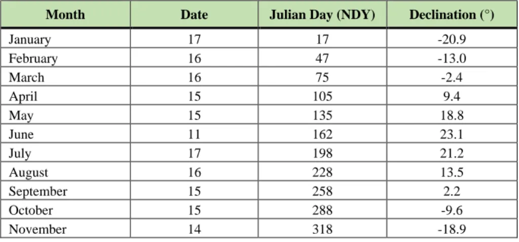
January (the Julian Day) as NDY (Table 1).

G

= G

×[1+0.033×cos(360/365×NDY)] (3) DEC refers to solar declination = 23.45×sin [(360/365) × (284+NDY) (4)

SSH denotes sunset hour angle = arcos (-tan Lat × tan Dec) (5)

Table 1. Recommended average day for each month and values of Julian day by month (Duffie

& Beckman, 2013)*

Month Date Julian Day (NDY) Declination (°)

January 17 17 -20.9

February 16 47 -13.0

March 16 75 -2.4

April 15 105 9.4

May 15 135 18.8

June 11 162 23.1

July 17 198 21.2

August 16 228 13.5

September 15 258 2.2

October 15 288 -9.6

November 14 318 -18.9

December 10 334 -23.0

* The average day which has the extra-terrestrial radiation closest to the average day for the month.

2.2 Photovoltaic Location Analysis

Potential shaded areas on a building envelope can be easily determined by visualizing the estimated solar energy density in three-dimensional (3D) colour rendering rather than by displaying it through mathematical calculation. The insolation received by the building envelope will be associated with surface colour where red represents the highest and blue refers the lowest insolation value. A bright-red colour indicated that the area of the envelope was less shaded while the dark-blue colour showed severely shaded areas. From this coloured envelope, the optimal placement for photovoltaic installation can be determined immediately.

BIM Revit software was used to construct 3D Models and to visualize incident solar radiation (insolation) that falls on the building envelope by employing the built in solar analysis tool. Location of photovoltaic panels was determined using monthly cumulative insolation received by the building envelope (walls and roof). Climate data including solar radiation data used in BIM Revit software was accessed through a cloud server called the Autodesk Climate Server that compiles data from both physical weather stations (at airports) and from meteorological simulations.

The incident solar radiation calculation in BIM Revit is computed as:

Incident solar radiation = (I

x F

x cos(Ɵ) + (I

x F

)+ I

(6) Where: I

refers to direct beam radiation, measured perpendicular to the sun, I

refers to diffuse sky radiation, measured on a horizontal plane, I

refers to radiation reflected from the ground, F

is the shading factor (1 if a point is not shaded, 0 if a point is shaded, a percentage if measured on a surface), F

denotes the visible sky factor (a percentage based on the shading mask), and Ɵ denotes the angle of incidence between the sun and the surface being analysed.

The simulation was conducted in three selected months; March, June, and December. These months represent the nearest and the farthest sun position towards the earth sky.

2.3 Area of Photovoltaic Placement Analysis

A guide to the basic available solar energy usually estimated by total annual solar radiation on a tilted surface is used so that the output is maximised. Energy generation from photovoltaic installation is often calculated from the following expression (Lang, Ammann, & Girod, 2016;

Mandalaki, Papantoniou, & Tsoutsos, 2014):

P

= G.η.PR.β.A (7)

Where, G refers to horizontal irradiance (Wh/m2), η denotes module efficiency, PR denotes performance ratio of the complete system before temperature effect, β refers to correction factor compared to a horizontal panel, and A refers to total panel area.

Electrical energy generation from photovoltaics is calculated for three

types of solar technology in this study, monocrystalline, polycrystalline and

amorphous silicon (Table 2). While several researchers estimated the

photovoltaic potential of power generation based on total annual solar

Equator line (0º) Palu

Jakarta

Bali

radiation (Lang, Ammann, & Girod, 2016; Mondal & Islam, 2011), this study uses a monthly calculation in order to investigate PV power generation within different months.

The potential of energy output from photovoltaics can be calculated per unit area (m² ) with area (A) equal to 1, so the expression will be:

P

= G.η.PR.β (8)

The area needed for photovoltaic placement on the building envelope to fulfil energy demand by the residential building can be drawn by dividing actual energy consumption with potential energy generation per unit area.

A

= E

/ P

(9)

Where, A

refers to the needed area for fulfilling energy demand, E

denotes actual energy consumption, and P

indicates generated electrical power by installed photovoltaic per unit area.

Table 2. PV Technology Efficiency used in Calculation

PV Technology Efficiency Power

deviation

Performance Ratio

Monocrystalline silicon 15% ± 3% 0.933

polycrystalline silicon 12% ± 3% 0.941

Amorphous silicon (thin film cells) 5% ± 5% 1.046

Adapted from (Lukač et al., 2014; Jelle, Breivik, & Røkenes, 2012).

2.4 Case Study: Palu City, Indonesia

Palu is located in the centre of Sulawesi Island which is one of the biggest islands in Indonesia. It is astronomically situated between 0.36º S – 0.56º S latitude and 119.45º E – 121.01º E longitude, with 0 – 700 m height above sea level (Figure 2). The climatic conditions in this area are categorized as tropical warm and humid climate. The city covers a total land area about 395.06 km² and is inhabited by 342,754 people.

Population growth in Palu has risen from 313 in 2009 to 356 people in 2013. At the same time, electrical energy consumption also rose from 297.59 GWh to 512.67 GWh. Accordingly, population rate had increased about 3%

while the energy consumption rate increased sharply, reaching 15% within these periods. As for many areas in Indonesia, the residential sector is the largest sector of electricity consumption in Palu. It was recorded in 2014 that the residential sector used 65% of total electrical energy generation, and this

Figure 2. Palu location in Indonesia archipelago

kept increasing each year. In 2005 residential buildings used 150.23 GWh of electrical energy and in 2014 it had doubled up to 382.34 GWh.

2.5 Solar Model

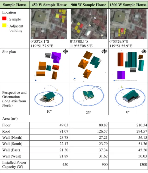
A solar model was contructed using Revit 2016 software. This model is used to determine and visualize the optimal location of photovoltaic installation within the building envelope. The constructed models are only based on three existing residential buildings in Palu City, which represent three different installed electrical energy generation systems, namely: 450, 900 and 1300 Watt systems (Table 3). No 2200W or 3500-6600W houses agrees to be objects of the study due to privacy reasons. Location data of the solar models and their obstruction from adjacent buildings based on the real existing location of the sample houses is as shown in Table 3.

Table 3. Sample Houses as Solar Models

Sample House 450 W Sample House 900 W Sample House 1300 W Sample House Location

: Sample : Adjacent

building

0°53'28.1"S 119°51'57.9"E

0°53'08.1"S 119°52'08.5"E

0°53'29.8"S 119°51'55.9"E Site plan

Perspective and Orientation (long axis from North)

10º 25º 0º

Area (m

)

Floor 49.03 80.87 210.34

Roof 81.07 126.57 294.57

Wall (North) 23.78 27.21 56.15

Wall (South) 22.17 23.79 51.36

Wall (East) 21.30 37.34 45.26

Wall (West) 21.89 31.62 50.03

Installed Power

Capacity (W) 450 900 1300

3. RESULT AND DISCUSSION 3.1 Solar Potential

The first step of analysis began with investigating solar potential for electrical energy generation. It was analyzed using global horizontal irradiation and average sunshine duration in different months. Total horizontal irradiation in Palu ranged from 168 – 202 kWh/m² per month with sunshine duration of 6 – 8 hours per day. The highest irradiation and the longest duration of sunshine happened in October, while the lowest level of irradiation and the shortest duration was in January (Figure 3). This condition was relatively varied by sunshine duration and cloud cover, which is clear in the lower rainfall period (October – December) and becomes cloudy in the rainy season (January – March). Inspite of the sky condition, variation of solar potential in the study case area is evenly distributed throughout the months.

The potential generated energy per unit area by photovoltaic installation with different levels of efficiency can be seen in Figure 4. Power output expected from monocrystalline, polycrystalline and amorphous sillicon ranges between 20 – 23 kWh/m² , 16 – 19 kWh/m² , and 7 – 9 kWh/m² respectively.

Thus, there is a promising potential for electrical energy supply from PV panels to fulfill self-energy demand for residential buildings.

0 2 4 6 8 10 12

0 25 50 75 100 125 150 175 200 225

Jan Feb Mar Apr Mei Jun Jul Ags Sep Okt Nop Des Average Sunshine Duration (hours)

Solar Radiation (kWh/m²)

Hor. Irradiance Sunshine Duration

Figure 3. Horizontal (Hor.) Global Irradiance in Case Study Location

0 50 100 150 200 250

0 5 10 15 20 25

1 2 3 4 5 6 7 8 9 10 11 12

Horizontal Irradiance (kWh/m2)

Potential of PV Output (kWh/m2)

mono.crst sillicon Poly.crst sillicon Thin-film Hor. Irradiance

Figure 4. Potential of Photovoltaic Energy Generation by Different PV

Technology

3.2 Residential Energy Consumption

The average electrical energy consumption data from 836 households was used and it varied from 264 – 328 kWh. The highest consumption was 2,280 kWh, and the lowest was 50 kWh (Figure 5) depending on the number of occupants, number and type of appliances, consumer behaviour and building area. The energy consumption from residential sectors was divided into five categories of installed electrical power capacity namely: 450W, 900W, 1300W, 2200W and 3500-6600W. The energy consumption data was gathered from State Electricity Enterprises data in 2015 and included 294 houses for 450V houses, 335 houses for 900W, 130 houses for 1300W, 59 data for 2200W and 18 houses for 3500-6600W.

This installed electricity generation capacity was generally representing the economic situation and the size of the detached house as well as the type of electrical appliances used in the house. But all these indicators came out of

y = 37.498x^1.0086 R² = 1

y = -1.5825x²+ 51.062x + 31.665 R² = 0.9955

y = 10.483x^1.558 R² = 0.9999

0 200 400 600 800 1,000 1,200 1,400

Energy Consumption (MWh)

Year

Residential Forecast(Residential)

Lower Confidence Bound(Residential) Upper Confidence Bound(Residential) Power (Forecast(Residential)) Poly. (Lower Confidence Bound(Residential)) Power (Upper Confidence Bound(Residential))

Figure 6. Predicted Residential Energy Demand in 2025 in Palu

Figure 5. Residential Energy Consumption by Installed Power Capacity in 2015

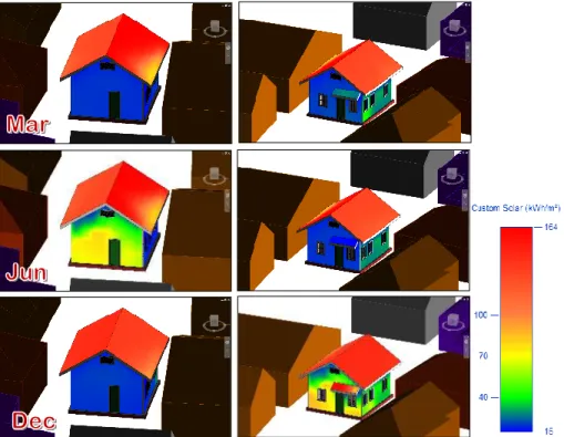
Figure 7. Solar irradiance falls onto building envelope of 450W building sample

discussion, except for the size of the building. The size of the building in this study refers to the surface area of the building envelope. This was used to evaluate the capacity of different types of power installed on a house to support their self-energy demand.

Ten years of average electrical energy consumption by residential sectors was used for projecting future energy demand in 2025 (Figure 6). From the projected energy consumption, it can be known that the energy demand in 2025 will be double the actual consumption in 2015. Accordingly, the monthly energy consumption data was multiplied by two to get the future monthly energy demand. The predicted value was used to calculate the area needed for a PV installation to supply sufficient electrical energy for the residential buildings self-energy demand for the next ten years.

3.3 Location of Photovoltaic Panel

Optimal location of photovoltaics was analysed by rendered colour visualization of superimposed insolation on the building envelope. As to be expected, the simulation result shows that three models receive the highest amount of solar energy on the roof, which always exceeds 100kWh/m² . This is due to their location in the equatorial region, thus the angle of the solar azimuth is near vertical for most months. Installing photovoltaics on the roof will provide a huge amount of electrical energy supply to the buildings.

The result of the 450W house model insolation coloured rendering can be seen in Figure 7. The figure shows that the insolation reached a maximum 164kWh/m² , shown by the bright-red colour of the associated roof surfaces.

On the contrary, heavily shaded walls resulted in the minimum insolation of

15kWh/m² which is represented by the dark-blue colour. The usable insolation

for photovoltaic installation in this study was determined to be from

50kWh/m² and higher.

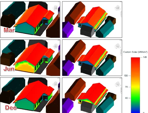
Figure 8. Solar radiation falls into building envelope of 900W building sample

The 450W model can receive a promising amount of solar radiation on its ESE facing wall throughout the year, displayed by a light green to yellow colour range (50-70kWh/m² ). SSW facing walls will receive a higher amount of solar radiation in December, displayed by the yellow to light-orange colour range which is between 70-90kWh/m² , while for the remaining months it only receives between 20 and 40 kWh/m² , displayed by the dark-green to green colour range (Figure 7). In contrast, NNE walls will receive higher insolation in June, rendered as yellow to orange in colour, representing an insolation value of 70 – 100kWh/m² , while the other months will receive a low insolation range 15 - 20kWh/m² . The lowest insolation received by NWN walls was due to being heavily obstructed by adjacent buildings, hence all the months are presented in blue colour.

.

Coloured rendering result for the 900W house model is showed in Figure 8. The bar scale of rendered colours displays the minimum insolation received by this model as 1 kWh/m² presented by the dark-blue colour, while the maximum value was 161 kWh/m² , the bright-red colour, which was achieved by roof surfaces. The model receives the highest amount of solar energy from SE facing walls especially in December. The amounts range from 80 to 100 kWh/m² in December and 50 – 65 kWh/m² for the remaining months. This is due to its orientation which is 25º from North, thus it receives higher radiation from the east circumsolar in the morning and south inclined circumsolar in December. Additionally, without any obstruction from adjacent construction, SE walls can gain more insolation than other walls of differing orientations.

The NW facing wall also received a promising potential in gaining electrical energy. The range of rendered insolation colours shown for this wall represent values of 40 – 65 kWh/m² . The NW walls received less insolation than SE walls because the available obstruction comes from near buildings.

On the other side, the NE facing wall receives unstable solar radiation. In June,

most parts of it received a higher amount (60 – 75 kWh/m² ) and the last part

only received 20 kWh/m² .

In the case of the 1300W model, three walls did not receive uniform amounts of solar radiation (Figure 9). This condition is due to its long axis facing exactly through North – South in orientation. Hence, solar radiation can only be received by North walls in June, and the South wall in December. This condition is worsened by the adjacent building which is too close to the model.

Better performance conditions are found for the East walls, where the amount of solar radiation varied from 50 kWh/m² to 70 kWh/m² . Enough space between the model and adjacent buildings on the East side allows morning solar radiation to reach East wall surfaces.

From the result of 3D insolation colour rendering, it can be seen that different building orientations have no major influence on the amount of insolation received by the roof element. Therefore, building orientation is not a critical factor for roof mounting of photovoltaics in the equatorial region.

On the contrary, the adjacent buildings’ height and distance indeed has significant influence, since adjacent structures can reduce the total amount of insolation received by the roof element by shading it. Shaded areas of roof also can be formed by its own construction. This study confirmed that the more complicated the roof form is, the less solar energy can be harvested due to self-shading of the roof element.

The optimal location of wall photovoltaic mounting is on the West and East walls. They not only provide a uniform solar energy distribution in different months, but also supply a higher amount of solar energy. Because these walls get the highest insolation, they also provide the highest potential for heat gain to the building interior. The higher the radiation amount falling onto the building envelope the more heat it produces, thus, potentially leading to overheating of interior environment. In the tropics, heat is a major problem for thermal comfort. Adding photovoltaic panels to both walls will add extra insulation to the walls.

Figure 9. Solar radiation falls into building envelope of 1300W model

3.4 Area of Photovoltaic Placement

Area of photovoltaic placement on the surfaces of the building envelope is mapped based on required size of photovoltaic installation area to support future energy demand. The result of the required area for each installed power capacity can be seen in Figures 10 –14. The highest value of required photovoltaic area across all months was selected for determining the area of photovoltaic placement on the building envelope.

To supply the average energy demand of the 450W model which ranges from 396 kWh to 512 kWh, the required area for photovoltaic placement using different technology was 66 m² for amorphous silicon, 31 m² for polycrystalline silicon, and 20 m² for monocrystalline silicon (Figure 10). The available roof area for this model is 81 m² , hence the roof surfaces alone are more than enough to fulfil the energy demand. For optimal energy generation, the shaded area by the adjacent building can be avoided for the photovoltaic placement. Therefore, the net area used for photovoltaic installation will be less than 81 m² which is 74.73 m² (Figure 10). This net area for the 450W model is still enough to serve the energy demand.

Available roof area on model 900W is 126.57 m² , while the required area is 83 m² , 38 m² , and 21 m² for amorphous silicon, polycrystalline silicon, and monocrystalline silicon respectively (Figure 11). 8.24 m² of this model’s roof surface area is shaded by its own form, making the net area available for photovoltaic installation 118.33 m² . With the remain net surface area, this model still surpasses the required area to serve the average energy demand of 497 – 612 kWh.

The average energy demand for the 1300W mode ranges from 603 – 728 kWh, thus the required area for photovoltaic mounting is 28 m² , 46 m² , and 99 m² for monocrystalline silicon, polycrystalline silicon, and amorphous silicon

Figure 10. Required area for photovoltaic installation on 450W model (left) and annual insolation mapped on building envelope (right)

Figure 11. Required area for photovoltaic installation on 900W model (left) and annual insolation mapped on building envelope (right)

0 10 20 30 40 50 60 70 80

Jan Feb Mar Apr May Jun Jul Aug Sep Oct Nov Dec

Area needed for PV installation (m²)

Area 450W Mono Area 450W Poly Area 450W Thin

0 10 20 30 40 50 60 70 80 90 100

Jan Feb Mar Apr May Jun Jul Aug Sep Oct Nov Dec

Area required for PV installation (m²)

Area 900W Mono Area 900W Poly Area 900W Thin

respectively (Figure 12). The available roof area is 284.57 m² , while the shaded area covers 49.74 m² of roof area. Hence, the remaining net roof surface area is 244.74 m² , which can adequately generate energy to supply future energy demand.

The simulated model for 2200W and 3500-6600W installed power capacity was not constructed. The reason is because none of the house owners from these types agreed to be measured as a study sample due to privacy reasons. This type of house belongs to the high-end economic class people.

Thus, the size of the houses is generally bigger than for the other types. The surface area of the houses is believed to meet the required area needed for photovoltaic installation. The required area for 2200W houses to supply an energy demand of 906 – 1176 kWh is 160 m² , 74 m² , and 44 m² for the three different photovoltaic technologies. While the required area for 3500-6600W houses to support an energy demand of 1485 – 1972 kWh is 75 m² , 120 m² , and 259 m² for monocrystalline silicon, polycrystalline silicon, and amorphous silicon respectively.

From the three models, it can be known that the available surface areas of the building envelope are more than enough to provide a sufficient amount of energy demand in the equatorial region. Available roof area alone from each model can suffice their own future energy demand. Therefore, photovoltaic mounting on residential building envelopes generally has excellent potential to supply the future energy demand.

4. LIMITATIONS

Our simulated models might be constrained by weather data which was accounted for by 5-yearly average values, and cannot account for short-term

0 50 100 150 200 250 300

Jan Feb Mar Apr May Jun Jul Aug Sep Oct Nov Dec

Area required for PV installation (m²)

Area 3500-6600W Mono Area 3500-6600W Poly Area 3500-6600W Thin 0

25 50 75 100 125 150 175 200

Jan Feb Mar Apr May Jun Jul Aug Sep Oct Nov Dec

Area required for PV installation (m²)

Area 2200W Mono Area 2200W Poly Area 2200W Thin

Figure 12. Required area for photovoltaic installation on 1300W model (left) and annual insolation mapped on building envelope (right)

Figure 13. Required area for photovoltaic installation on 2200W and 3500-6600W electrical power installed capacity houses

0 20 40 60 80 100 120

Jan Feb Mar Apr May Jun Jul Aug Sep Oct Nov Dec

Area required for PV installation (m²)

Area 1300W Mono Area 1300W Poly Area 1300W Thin

weather variation. The building models also might not resemble all residential buildings in Palu City. In addition, this prediction only focuses on the available area from the building envelope surfaces for photovoltaic mounting, thus giving rise to several interesting points for future research. First, our study models only consider solar radiation gained by photovoltaic panels for energy output calculations, therefore temperature effect behaviours of the photovoltaic panels become an interesting future research topic, especially in tropical climates. Second, economic consideration should be included in assessments of prospective photovoltaic building installations. Finally, extending the study scope from single buildings to neighbourhoods and entire areas will become a future point of study.

5. CONCLUSION

In this paper, we evaluated the potential of photovoltaic installations on residential building envelopes in the equatorial region by constructing three buildings, representing three different categories of electricity generation in BIM Revit software. Our study proposes a practical method for photovoltaic potential evaluation employing 3D insolation colour rendering which can be easily implemented at the building design stage by building designers. The method included optimal area on the building envelope to provide sufficient electrical energy for future energy demand.

Evaluation results show that implementation of photovoltaics on residential building envelopes has enormous potential in the equatorial region.

Roof surfaces of residential buildings can have photovoltaics attached, for the highest and relatively uniform amount of solar radiation falls onto this area throughout the year. Walls of the building oriented to East and West also have great potential to harvest electrical energy. Additional barriers to the effectiveness of wall-mounted photovoltaics are the surrounding obstruction, like buildings, though trees have enough space for solar radiation to penetrate to the walls.

To design new buildings with optimal PV power generation, a simple roof design and a building form that avoids self-shading potential is highly recommended. Larger wall areas may be oriented to East and West as additional areas for PV installation, however, thermal loading to a residence needs to be considered.

ACKNOWLEDGMENTS

The authors are grateful to JSPS (C) for providing funding through the Urban Planning Laboratory (project no. 15K06354), Kanazawa University.

The authors also would like to thank the Directorate of Higher Education, Ministry of Research and Higher Education of Indonesia for supporting this research.

REFERENCES

Adaramola, M. S. (2014). "Viability of Grid-Connected Solar Pv Energy System in Jos,

Nigeria". International Journal of Electrical Power & Energy Systems, 61, 64-69. Retrieved

from http://www.sciencedirect.com/science/article/pii/S0142061514001173.

Brock, T. D. (1981). "Calculating Solar Radiation for Ecological Studies". Ecological modelling, 14(1-2), 1-19.

Duffie, J. A., & Beckman, W. A. (2013). Solar Engineering of Thermal Processes. (4th ed.).

New Jersey: John Wiley & Sons. Retrieved from

https://books.google.co.jp/books?id=Q1tjDQAAQBAJ.

El-Shimy, M. (2009). "Viability Analysis of Pv Power Plants in Egypt". Renewable Energy, 34(10), 2187-2196. Retrieved from http://dx.doi.org/10.1016/j.renene.2009.01.010.

Fath, K., Stengel, J., Sprenger, W., Wilson, H. R., Schultmann, F., & Kuhn, T. E. (2015). "A Method for Predicting the Economic Potential of (Building-Integrated) Photovoltaics in Urban Areas Based on Hourly Radiance Simulations". Solar energy, 116, 357-370.

Retrieved from http://dx.doi.org/10.1016/j.solener.2015.03.023.

Gupta, A., Cemesova, A., Hopfe, C. J., Rezgui, Y., & Sweet, T. (2014). "A Conceptual Framework to Support Solar Pv Simulation Using an Open-Bim Data Exchange Standard".

Automation in Construction, 37, 166-181.

Ham, Y., & Golparvar-Fard, M. (2015). "Mapping Actual Thermal Properties to Building Elements in Gbxml-Based Bim for Reliable Building Energy Performance Modeling".

Automation in Construction, 49, 214-224.

Hofierka, J., & Kaňuk, J. (2009). "Assessment of Photovoltaic Potential in Urban Areas Using Open-Source Solar Radiation Tools". Renewable Energy, 34(10), 2206-2214.

Jelle, B. P., Breivik, C., & Røkenes, H. D. (2012). "Building Integrated Photovoltaic Products:

A State-of-the-Art Review and Future Research Opportunities". Solar Energy Materials and Solar Cells, 100, 69-96.

Koenigsberger, O., Ingersoll, T., Mayhew, A., & Szoklay, S. (1974). Manual of Tropical Housing and Building: Climatic Design. London, UK: Longman. Retrieved from https://books.google.co.in/books?id=l-I4AQAAIAAJ.

Kuo, H.-J., Hsieh, S.-H., Guo, R.-C., & Chan, C.-C. (2016). "A Verification Study for Energy Analysis of Bipv Buildings with Bim". Energy and Buildings, 130, 676-691.

Lang, T., Ammann, D., & Girod, B. (2016). "Profitability in Absence of Subsidies: A Techno- Economic Analysis of Rooftop Photovoltaic Self-Consumption in Residential and Commercial Buildings". Renewable Energy, 87, 77-87.

Lukač, N., Seme, S., Žlaus, D., Štumberger, G., & Žalik, B. (2014). "Buildings Roofs Photovoltaic Potential Assessment Based on Lidar (Light Detection and Ranging) Data".

Energy, 66, 598-609.

Mandalaki, M., Papantoniou, S., & Tsoutsos, T. (2014). "Assessment of Energy Production from Photovoltaic Modules Integrated in Typical Shading Devices". Sustainable Cities and Society, 10, 222-231.

Markus, T. A., & Morris, E. N. (1980). Buildings, Climate, and Energy. London: Pitman Publishing. Retrieved from https://books.google.co.jp/books?id=skm0AAAAIAAJ.

Matrawy, K., Mahrous, A.-F., & Youssef, M. (2015). "Energy Management and Parametric Optimization of an Integrated Pv Solar House". Energy Conversion and Management, 96, 377-383.

Mondal, M. A. H., & Islam, A. S. (2011). "Potential and Viability of Grid-Connected Solar Pv System in Bangladesh". Renewable Energy, 36(6), 1869-1874.

Othman, A. R., & Rushdi, A. T. (2014). "Potential of Building Integrated Photovoltaic Application on Roof Top of Residential Development in Shah Alam". Procedia-Social and Behavioral Sciences, 153, 491-500.

Seng, L. Y., Lalchand, G., & Lin, G. M. S. (2008). "Economical, Environmental and Technical Analysis of Building Integrated Photovoltaic Systems in Malaysia". Energy Policy, 36(6), 2130-2142.

Shan, F., Tang, F., Cao, L., & Fang, G. (2014). "Comparative Simulation Analyses on Dynamic Performances of Photovoltaic–Thermal Solar Collectors with Different Configurations".

Energy Conversion and Management, 87, 778-786.

Szokolay, S. V. (1987). Thermal Design of Buildings. Canberra: RAIA Education Division.

Vieira, F. M., Moura, P. S., & de Almeida, A. T. (2017). "Energy Storage System for Self- Consumption of Photovoltaic Energy in Residential Zero Energy Buildings". Renewable Energy, 103, 308-320.

Vuong, E., Kamel, R. S., & Fung, A. S. (2015). "Modelling and Simulation of Bipv/T in Energyplus and Trnsys". Energy Procedia, 78, 1883-1888.

Yoza, A., Yona, A., Senjyu, T., & Funabashi, T. (2014). "Optimal Capacity and Expansion

Planning Methodology of Pv and Battery in Smart House". Renewable Energy, 69, 25-33.