Uniaxial Loading by X-ray CT Method

Uniaxial Loading by X-ray CT Method

Yuzo Obara, Izumi Tanikura Jahe Jung , , Ren Shintani

Journal of Advanced Concrete Technology, volume ( ), pp. 14 2016 433-443 Shinya Watanabe ,

Characterizing the 3D Pore Structure of Hardened Cement Paste with Synchrotron Microtomography Michael $% Promentilla , Takafumi Sugiyama Takashi Hitomi , , Nobufumi Takeda

Journal of Advanced Concrete Technology, volume ( ), pp. 6 2008 273-286

X-ray microtomography of mortars exposed to freezing-thawing action Michael A. B. Promentilla , Takafumi Sugiyama

Journal of Advanced Concrete Technology, volume ( ), pp. 8 2010 97-111

Application of X-ray CT to study diffusivity in cracked concrete through the observation of tracer transport

Ivan Sandi Darma, Takafumi Sugiyama Michael , $% Promentilla

Journal of Advanced Concrete Technology, volume ( ), pp. 11 2013 266-281

Scientific paper

Evaluation of Micro-damage of Concrete Specimens under Cyclic Uniaxial Loading by X-ray CT Method

Yuzo Obara

*, Izumi Tanikura

, Jahe Jung

, Ren Shintani

and Shinya Watanabe

Received 28 Nobember 2015, accepted 8 August 2016 doi:10.3151/jact.14.433

Abstract

The X-ray CT method was applied to evaluate micro-damage – namely, deterioration of concrete specimens under cyclic uniaxial loading tests. The μ-focus X-ray CT scanner was used. Concrete cylinders with a diameter of 50 mm and a length of 100 mm were prepared as specimens. Cyclic uniaxial loading tests were conducted on the specimens. The X-ray CT images of the specimens were taken at the loading level 0, 60, 70, 80 and 90 percent of their uniaxial com- pressive strength. For three dimensional CT images of the specimen, the Three Dimensional Medial Axis Analysis (3DMA) method was applied to evaluate porosity and width, length, persistence of cracks which represent deterioration of the specimen. As the results, slight micro-fracturing occurs until a loading level R = 60%, and starts to increase at R of 60% to 70%. The cracking occurs in a part of the mortar near boundary between aggregate and mortar, and the crack links to another crack with increasing loading level. The degree of cracking varies according to the position dependent on the final apparent fracture surface of the specimen. It is concluded that the X-ray CT method with 3DMA is effective for not only evaluating the state of micro-cracking within the specimen, but also estimating the process of deterioration of the specimen with an increasing loading level.

1. Introduction

It is known that a concrete consists of aggregate, mortar and defects like pores. Accordingly, the concrete is a heterogeneous and anisotropic material on a microscopic scale. On the other hand, the mechanical property of concrete is dependent on the mix proportion of wa- ter-to-cement ratio, grain size distribution of aggregate, kind of aggregate, and cement. When stress acts on such concrete, microscopic damage within it progresses gradually and macroscopic fractures developed. It is important to make clear the process of micro-damage to apparent fracture for understanding the relation between microstructure and mechanical properties. Especially, experimental evaluation of the micro-damage is indis- pensable because concrete is a heterogeneous and ani- sotropic material.

In order to evaluate micro-damage of brittle materials such as rocks and concrete due to loading, various studies have been conducted using several different methods

such as the Acoustic Emission (AE) method, fluorescent method and X-ray CT method.

The AE method is used to analyze not only the loca- tion of cracking but also type of cracking of concrete and rock during loading, using arrival time and energy of an elastic wave caused by micro-cracking measured by sensors attached on the surface of specimen (Ohtsu et al.

1998; Abdelrahman et al. 2014). However, it is difficult to estimate width, length, and persistence of the cracks by the AE method. The fluorescent method is one of the techniques to observe and quantify micro-cracks within a specimen by image analysis after injecting fluorescent paint to micro-cracks. Wajima et al. (2000) and Chen et al. (2015) visualized microscopic pore spaces and mi- cro-cracks filled with synthetic resin mixed with fluo- rescent paint under ultraviolet light for oil, gas, and geo- thermal reservoir rocks. However, since a specimen is cut or a thin section is made from the specimen, the results of the method are described in two dimensions.

On the other hand, the X-ray CT method is one of the nondestructive methods to investigate the internal structure within a material by re-constructed three di- mensional images regarding X-ray attenuation coeffi- cient. The first application of X-ray CT method to geo- materials was in soil mechanics (Anderson and Hopmans 1992; Aylmore 1994; Hopmans et al. 1994). The first international workshop of X-ray CT for geomaterials - Soils, Concrete, & Rocks - Geo-X 2003 (Otani and Obara 2003) - was held at Kumamoto in 2003. From that same period, many papers for application of X-ray CT to geometerials could be found in international journals.

Especially for mortar and concrete, Landis et al. (2000) applied X-ray CT to mortal, then discussed relation be- tween fracture energy and induced crack area in com-

1

Professor, Graduate School of Science and Technology, Kumamoto University, Kumamoto, Japan.

*Corresponding author,

E-mail: [email protected]

2

General Manager, Japan Construction Method and Machinery Research Institute, Shizuoka, Japan.

3

Research Engineer, Korea Institute of Civil Engineering and Building Technology, Seoul, Korea.

4

Master Student, Graduate School of Science and Technology, Kumamoto University, Kumamoto, Japan.

5

Senior Researcher, Japan Construction Method and

Machinery Research Institute, Shizuoka, Japan.

pression test. Landis et al. (2003) also applied to concrete, then the fracture within a specimen was visualized and fracture energy was analyzed under cyclic uniaxial compression test. Wang et al. (2003) visualized voids or cracked surfaces using X-ray CT, and suggested a dam- age tensor for representing damage. Elaqra et al. (2007) explores the use of acoustic emission (AE) and X-ray tomography to identify the mechanisms of damage and the fracture process during compressive loading on mortar specimens. Recently, Sugiyama et al. (2010) applied the synchrotron X-ray CT at Spring 8 with a resolution of 0.5μm to the deteriorated mortal, then visualized pore space and made clear diffusion tortuosity in the pore evaluated by random walk simulation.

Promentilla and Sugiyama (2010) applied micro-focus X-ray CT to characterization of internal structure of mortal exposed by freezing-thawing action, then made clear void function, air void size distribution, crack width and tortuosity of connected crack network in three di- mensions. Application of X-ray CT to estimating diffu- sivity in cracked concrete was performed by Darma et al.

(2013). In the research, cesium carbonate solution was used as a tracer, the diffusion from a fracture to concrete was discussed. Ren et al. (2015) and Huang et al. (2015) suggested two-dimensional and three-dimensional meso-scale finite element models of concrete based on X-ray CT images to make clear complicated damage and fracture behavior respectively. Tian et al. (2015) also tried to quantify the internal meso-cracking of concrete for estimating damage under a uniaxial compression test using a helical CT scanner. However, most research regarding damage to concrete using the X-ray CT method focused on apparent fractures produced within the specimen and post peak stress in a cyclic uniaxial compression test, and there has been little research to treat micro-cracking before peak stress. Jung et al.

(2014) demonstrated the quantitative analysis of internal micro-cracking of a concrete specimen during cyclic uniaxial compression testing before the apparent fracture surfaces are produced within the specimen, using three-dimensional X-ray CT imaging.

The objective of this paper is to establish a nonde- structive method of evaluating micro-damage in a con- crete specimen before the apparent fracture surfaces are produced within it. For this purpose, a μ-focused X-ray CT scanner was used to investigate the internal structure of concrete, especially its state of micro-cracking. Firstly, the cyclic uniaxial loading test is performed on a con- crete specimen with a diameter of 50 mm and a length of 100 mm. X-ray CT images of the specimen which ex- perienced each loading step are taken after loading.

Subsequently, the Three Dimensional Medial Axis Analysis (3DMA) (Lindquist et al. 1996, 1999) is ap- plied to the three-dimensional CT data of the specimen.

The porosity P

, burn number and medial axis of the parameters in the 3DMA are used in order to represent micro-damage to the specimen. Analyzing the porosity, the voxel count of the burn number, and the

three-dimensional medial axis of cracks at each loading level, it is made clear that the deterioration of the specimen can be estimated quantitatively. As a result, it was shown through analysis by 3DMA that the new micro-cracks are induced and the porosity increases with increasing applied cyclic load. Consequently, it was concluded that the X-ray CT method with the 3DMA is available for evaluating the porosity and the burn num- ber which are parameters of the deterioration estimation of the specimen.

2. X-ray CT scanner and CT image

The μ-focused X-ray CT scanner is used in this research at the X-Earth Center of Kumamoto University. An il- lustration of the inner view and its specifications are shown in Fig. 1 and Table 1. A flat panel detector (FPD) is utilized to perform a three-dimensional scan with an X-ray cone beam. Figure 2 is a view of a scan in the

Table 1 Specification of μ-focused X-ray CT scanner.

Radiographic field of vision 400 mm, height 500 mm Number of display pixels Cone 1024×1024

Resolution 5 μm minimum

Cone beam scan Normal, Offset, Half

X-ray beam thickness 5 μm minimum

Power of X-ray 240 kV (140 W) maximum

Maximum sample weight 245 N

ﾏｲｸﾛ･ﾌｫｰｶｽＸ線発生装置

FPD：X軸移動

ｽｷｬﾝﾃｰﾌﾞﾙ：

X,Y,Z軸移動

X-ray tube

FPD Specimen table

Fig. 1 Schematic of the μ-focus X-ray CT system.

X-ray tube

Specimen

Specimen table

Fig. 2 View of scan in the shield room.

μ-focused X-ray CT shield room. Once a specimen is set up on the specimen table, a cone-shaped X-ray beam is emitted from an X-ray tube and the specimen is scanned.

During the scanning, only the specimen table is rotated during scanning so that the X-ray beam can penetrate the specimen from 360 degrees (Mukunoki et al. 2011). The scan condition in this study: voltage is 150 kV, current is 200 μA, slice pitch is 50μm, and slice thickness is 50 μm.

Therefore, the voxel dimension of the X-ray CT image is 50 × 50 × 50μm.

Figure 3 shows a two dimensional X-ray CT image of a specimen with a diameter of 50 mm. This image is constructed of cubic voxels with 1024 × 1024 pixels with a dimension of 50 × 50 × 50μm. The CT value of each voxel is calculated in eq. (1):

CT value = K μ + L (1)

where μ

is the X-ray absorption coefficient of a re- quired point. K and L are constants which depend on the scan condition such as voltage and current. In this study, these constants are unchanged because that scan condi- tion is the same at every scans.

The concrete specimen consists of aggregate, mortar, and pores, as shown in Fig. 3(a). Those are distin- guished in the CT images by the differences between light and shade (gray scale image). The high density aggregate shows light gray, pores with low density are black, and mortar of medium density appears as dark gray. A three-dimensional X-ray CT image is recon- structed using many two-dimensional X-ray CT images.

3. Deterioration parameters

The Three Dimensional Medial Axis Analysis (3DMA) computational package is applied to analyze the geome- try of pores, cracks, fractures, and porosity in three-dimensional CT data. Parameters used in 3DMA to evaluate the degree of deterioration are porosity P

, burn number, and medial axis. It was revealed that those parameters were effective for evaluating width, length, persistence of cracks and fracture, and their distribution.

The parameter P

is the porosity on the image and de- fined by the percentage of number of pore voxels to total

number of voxels as eq. (2) in an area of the specimen.

idx

voxel count of pore

100(%) voxel count of analysis area

P = × (2)

The burn number and medial axis are explained using Fig. 4. Each pore voxel is assigned an integer describing its distance from the border of the aggregate. The ag- gregate voxel on the pore-aggregate surface is assigned distance 0. Each of its neighboring pore voxels are as- signed distance 1. Each of the neighbors of these distance 1 voxels which have not yet been assigned a distance are assigned distance 2. This algorithm is iterative, and an integer is assigned to all voxels. The value in each pore voxel is called burn number in this study. In pore voxels, the burn number represents a distance from a voxel placed on a boundary of the aggregate or mortar. In the case of cracking, it represents the width of the crack.

Therefore, the larger the burn number, the wider the width of the crack. In addition, as the burn number is one of parameters which indicate width of cracks, this pa- rameter was payed attention and the crack surface area was not treated in this paper.

The medial axis for a pore is a line passing through the center voxel. Therefore, a network of lines represents continuity of a pore, a crack, and a fracture. The de- tailed algorithm and definition of 3DMA are referred to by Lindquist et al. (1996, 1999) and Promentilla et al.

(2010).

4. Cyclic uniaxial loading test 4.1 Specimen

Concrete specimens with water to cement ratios of 30%

(W30), 50% (W50), 70% (W70) and 90% (W90) were prepared. The materials of the concrete are shown in Table 2. The mix proportion of the specimen is shown in

Table 2 Materials of concrete specimen.

Material name Materials Density(g/cm

)

Cement Ordinary Portland cement 3.16

Coarse aggregate River sand 2.66

Fine aggregate River sand, Ground sand 2.64 NOTE: Maximum size of coarse aggregate is 15mm.

Aggregate Pore

Air

1024x1024 Pixel (Pixel length: 5 µm)

Slice thickness:

(b) 5 µm

Pixel length : 5μm

1024Pixels

1024Pixels

Slice thickness:

Aggregate 5μm

(a) (b)

Fig. 3 X-ray CT image and voxel data: (a) X-ray CT image of the sample with a diameter of 50 mm, (b) number, length,

and height of pixels divided from image.

Table 3. Air entraining and a water reducing agent were used as the mixture. The workability is assured by using water reducing agent without AE agent. The diameter and height of the specimens were 50 mm and 100 mm respectively. After curing, those were placed in a dry oven of 40°C until the weight of the specimen no longer changed.

4.2 Cyclic uniaxial loading condition

The cyclic uniaxial loading tests are conducted using a material testing machine as shown in Fig. 5(a). The load and the displacement are measured by a load cell and a dial gauge, respectively in Fig. 5(b). The cyclic loading level was 60, 70, 80 and 90% of the uniaxial compressive strength of the specimens for each water-to-cement ratio.

The values were determined by a uniaxial compression test before the cyclic loading test. The loading level on each loading step is defined by eq. (3):

100(%)

c

R S

= σ × (3)

where, R is the loading level, σ is the applied stress, and S

is the uniaxial compressive strength of the specimen for each water-to-cement ratio. In this paper, R is defined as 60%, 70%, 80% and 90%. The CT images of the specimens were taken when the specimens were not loaded (i.e. initial state before loading) and unloaded after loading by each level. The stress-strain curves at each loading step are placed in Fig. 6. In the figure, ○

: X-ray CT image was taken in an initial (not loaded) state; ○

: X-ray CT image was taken after loading step of R=60%; ○

~ ○

: X-ray CT images were taken after loading step of R=70, 80 and 90%. Using the CT images, the deterioration of the specimen is analyzed at each loading step.

Table 3 Mix proportion of concrete specimen.

Unit weight (kg/m

) Sample No.

W/C content

(%)

Fine aggregate

ratio (%) Water Cement Fine

aggregate

Coarse aggregate

Water reducing

agent (kg) Air (%)

W30 30 48 165 550 785 856 5.50 0.6

W50 50 48 165 330 874 955 3.30 4.6

W70 70 48 165 236 911 995 2.36 3.5

W90 90 48 165 183 932 1019 1.83 1.7

(a) (b) (c)

Fig. 4 Burn number and medial axis: (a) X-ray CT image, (b) enlarged view consisting of aggregate, mortar, and pore, (c) burn number assigned in pore voxels and medial axis connecting voxels passing through the center point of a pore.

(a) (b)

Fig. 5 View of cyclic uniaxial loading test: (a) material testing machine, (b) a specimen with a load cell and a dial gauge.

5. Image analysis

5.1 Determination of threshold value

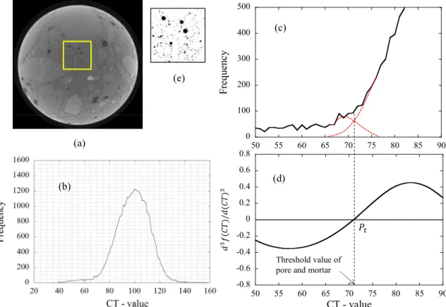
During cyclic loading, cracking occurs within the specimen, and deterioration progresses. As a result, po- rosity is considered to increase with increasing loading level. Therefore, the deterioration can be estimated by analyzing pores and cracks which are extracted from the CT image. For this purpose, the CT value histogram of a CT image in Fig. 7 (b) is used. This is the histogram in a

region of interest (ROI) with a square in Fig. 7(a). The vertical axis is the voxel count, and the horizontal is the CT value. The CT values which represent pores and cracks with lower density are distributed on the left side, mortar in the middle, and aggregate with higher density on the right side in the diagram. In order to differentiate among pores, cracks and others, a threshold value to represent the boundary between them should be deter- mined, and the CT image can be binarized by it.

When the distribution is a bimodal distribution of the histogram, its valley appears, and the threshold value is easily determined as being the bottom of the valley.

However, this characteristic cannot be found in the his- togram of the concrete specimen used in the test as shown in Fig.7(b). Therefore, the threshold value was determined using the third-order differential method of CT value diagram (Temmyo and Obara 2010).

An enlarged view near the CT value of the boundary between pore and mortar in the histogram is shown in Fig.

7(c). The voxel count in a range between 50 and 90 of the CT value clearly increases because the distributions of pore and mortar overlap in the range. Both distributions are represented as thin dotted lines in the figure, and the histogram is obtained by superposing these distributions.

However, the distribution near the intersection point of two distributions is not a monotone increasing function.

Therefore, third-order differential values of the original distribution are calculated. In this calculation, the origi-

R=80%

R=90%

Strain (10^-3) 20

40 60 80 100

0 1 2 3 4 5 6 7

Stress (MPa)

1

4 5 2 3

② ③ ④ ⑤

R=70%

R=80%

R=90%

①

Stress, MPa

Strain , 10

Fig. 6 Stress-strain curve and scan of X-ray CT at each loading step.

(a)

-0.8 -0.6 -0.4 -0.2 0 0.2 0.4 0.6 0.8

50 55 60 65 70 75 80 85 90

CT - value

100 200 300 400 500

50 55 60 65 70 75 80 85 90

Fre quenc y

(b)

(c)

(d) (e)

Fig. 7 Determining method of threshold value from the histogram of CT value and binarized image: (a) original X-ray im-

age, (b) histogram of CT vale of the regions of interest (ROI), (c) enlarged view and distributions of the histogram, (d)

determination of threshold value by the third-order differential method, (e) binarized image of ROI using the determined

threshold value.

nal function is approximated by a quadratic curve using 21 sequence data of CT-value and frequency, then a first-order differential vale is estimated at middle point of 21 data of CT-value using the approximated curve. Re- peating this procedure with increasing CT-value, a first-order differential function is obtained. Applying this procedure to the obtained data repeatedly, a third-order differential function can be obtained as shown in Fig.

7(d). The point at which the lateral axis and the function intersect almost coincides with the intersection point of distributions of pore and mortar. Consequently, the CT value at this point P

is adopted as a threshold value.

Using this value, the binarized image is obtained as shown in Fig. 7(e).

5.2 Three dimensional image construction The number of 2D X-ray CT specimen images is 1,800.

Three-dimensional (3D) image reconstruction is per- formed, and 3D volume data of whole specimen is shown in Fig. 8. The entire specimen was taken by X-ray CT scanner at each loading level. It is considered that the damages near upper and lower ends of it are affected by the restrained condition by loading platen. Therefore, in order to consider variability of damages in position, the discs at middle position of upper and lower parts within the specimen are selected. Then, as shown in Fig. 8(c), ROIs are chosen in the upper and lower part of the specimen, and five ROIs (area 1 ~ area 5) are set in each part, considering the expanse of damage within it. Each area is defined as a 10 mm cube for effective analysis.

The total number of voxels in an area is about 8 million.

The 3DMA is applied to each area in order to analyze the deterioration parameter: porosity, burn number, and dis- tribution of medial axis. In addition, choosing these areas inside position surrounded by a center circle having a diameter of about 30mm, the beam hardening can be avoided in the analysis. Because that the diameter of the specimen is 50mm.

6. Results and discussion

6.1 Typical example of change in burn number and medial axis

Figure 9 shows an example of analyzed results of area 2 in the upper part of W90. Figures 9(a), (b) and (c) show the medial axis distribution and the burn number for R=0%, 60% and 90%, respectively. The warm color is a small burn number and the cold color represents a large burn number in results of medial axis distribution. The red color represents burn number 1. The histogram of the burn numbers 1 to 5 are plotted on the right.

In the medial axis distribution for an initial condition of R=0%, small cracks represented by red appear. There is a relative large lump which is represented by yel- low-green in the lower right. This is a pore, not a crack.

The voxel count of burn number 1 is highest, reaching about 5,000 in the figure on the right. In the distribution at R=60%, the medial axes increase as a u-shaped curve along the surface of the analyzed cube area. Of course, there is the relative large lump at the same position at R=

0%. An aggregate is located at the blank space of medial axis in the upper part. The voxel count of burn number 1 increases to more than 10,000, and that of burn number 2 likewise increases. A large number of medial axes are drawn all over, except in the aggregate in the cube area, and the voxel count of burns number 1 and 2 increase. It is clear that cracking hardly occurs in aggregate and that most cracks are induced in the mortar part. The voxel count of all burn numbers increases with increasing loading level R. In particular, the increase of burn num- ber 1 was remarkable. This result indicates that cracks with a width of less than 0.1 mm increased due to loading and advanced the deterioration of the specimen. This phenomenon has already been seen in many experiments, but the three-dimensional visualization of it has not been investigated in detail. Such three-dimensional visualiza- tions were obtained in this study.

Figure 10 shows the voxel count of each burn number

900 sliced images

900 sliced images

3D volume data ROI for image analysis Overlaying

the sliced images

10mm 10mm

10mm 10mm

area1 area2 area3 area4

area5

(a) (b) (c) (d)

Fig. 8 3D reconstruction using the sliced CT images and analyzed area in the 3D volume data: (a) overlaying the sliced

images, (b) 3D volume data made by overlaying the sliced images, (c) location of analyzed area in upper and lower part of

the specimen, (d) definition of analyzed area.

with increasing loading level. The result at the loading level R=70% and R=80% are added with results shown in Fig. 9. The increase in voxel count of burn number1 is greatest with increasing loading level. Especially, the ratio of increase is remarkable from R=60% to 70%.

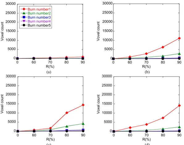
6.2 Change in burn number with loading level The changes in burn number with the loading level R are shown in Figs. 11 and 12. Both are results of the upper and lower parts of the specimen, respectively. The voxel count corresponding to each burn number is the mean value of those of five areas. Only results from burn numbers 1 to 5 are plotted.

The voxel count of all burn numbers increases with increasing loading level R. Especially, the change of burn number 1 increases from R=60%, and, after that, gradu- ally increases in both parts. That of burn numbers 3 to 5 is relatively small. It is shown that there are many mi- cro-cracks and minor damage within the specimen until R=90%.

Such a tendency is shown at the lower part of the specimen. However, the rate of increase of the voxel count of all burn numbers in the lower part is smaller than that in the upper part. In only W50, which is larger in the lower part, but those differences are slight. This

0 10000 20000 30000 40000 50000 60000

1 2 3 4 5

Voxel count

Burn Number R=0%

(a)

0 10000 20000 30000 40000 50000 60000

1 2 3 4 5

Voxel count

Burn Number R=60%

(b)

0 10000 20000 30000 40000 50000 60000

1 2 3 4 5

Voxel count

Burn Number R=90%

(c)

Fig. 9 Distribution of medial axis in area 2 of the upper part of W90: (a) R=0%, (b) R=60%, (c) R=90%.

0 10000 20000 30000 40000 50000 60000

0 60 70 80 90

Burn number1 Burn number2 Burn number3 Burn number4 Burn number5

Voxel count

R(%)

Fig. 10 Burn number in area 2 of the upper part of W90.

0 5000 10000 15000 20000 25000 30000

0 60 70 80 90

Burn number1 Burn number2 Burn number3 Burn number4 Burn number5

Voxel count

R(%)

0 5000 10000 15000 20000 25000 30000

0 60 70 80 90

Voxel count

R(%)

(a) (b)

0 5000 10000 15000 20000 25000 30000

0 60 70 80 90

Voxel count

R(%)

0 5000 10000 15000 20000 25000 30000

0 60 70 80 90

Voxel count

R(%)

(c) (d)

Fig. 11 Variation of mean value of each burn number of five areas depending on R (upper part): (a) W30, (b) W50, (c) W70, (d) W90.

0 5000 10000 15000 20000 25000 30000

0 60 70 80 90

Burn number1 Burn number2 Burn number3 Burn number4 Burn number5

Voxel count

R(%)

0 5000 10000 15000 20000 25000 30000

0 60 70 80 90

Vovel count

R(%)

(a) (b)

0 5000 10000 15000 20000 25000 30000

0 60 70 80 90

Voxel count

R(%)

0 5000 10000 15000 20000 25000 30000

0 60 70 80 90

Voxel count

R(%)

(c) (d)

Fig. 12 Variation of mean value of each burn number of five areas depending on R (lower part): (a) W30, (b) W50, (c)

W70, (d) W90.

means that a fracture within a specimen does not pro- gress uniformly. Figure13, from ASTM C 39-03,

“Standard Test Method for Compressive Strength of Cylindrical Concrete Specimens,” shows five different types of fracture after testing (American Concrete Insti- tution 2015). The fracture surfaces are produced in specimens of all types. In the cases of cone and split failure, cone and shear failure, the fracture surfaces are produced by forming different geometry in the upper and lower parts of the specimen. This means that the degree of deterioration in the lower part is larger than that in the upper part. This is compatible with the results in this study.

6.3 Change in porosity with loading level The changes in the porosity P

with the loading level R are shown in Figs. 14 and 15, which show results in the

upper and lower parts of the specimen, respectively. The mean values of five areas are plotted in the figures. In both parts, regardless of water-to-cement ratio, the values of P

were almost constant until R=60%, then increased moderately with increasing R. In the upper part, there are areas where P

decreased with increasing R, such as area 1 of the W50 and area 5 of the W70, and there are areas where P

did not change with increasing loading level, such as area 4 of the W30 and area 1 of the W50.

On the other hand, the difference of P

between R=0%

and R=90% in the results of the lower part is smaller than those of the upper part, but the tendency of increasing porosity in the lower part is similar to that in the upper part. Thus, the degree of deterioration varies according to the position, because that concrete is an inhomogeneous material composed of aggregate, mortar, and pores.

Considering the results of the burn number, the medial

Corn Corn and Split

Corn and Shear

Shear Columnar (a) (b) (c) (d) (e)

Fig. 13 Sketches of types of fracture.

0 2 4 6 8 10 12 14 16

0 20 40 60 80 100

area1 area2 area3 area4 area5 mean value

Porosity(%)

R(%)

0 2 4 6 8 10 12 14 16

0 20 40 60 80 100

Porosity(%)

(a) (b)

0 2 4 6 8 10 12 14 16

0 20 40 60 80 100

Porosity(%)

R(%)

0 2 4 6 8 10 12 14 16

0 20 40 60 80 100

Porosity(%)

(c) (d)

Fig. 14 Variation of the porosity (P

) values depending on R (upper part): (a) W30, (b) W50, (c) W70, (d) W90.

axis, and the porosity, the progress of failure within the concrete specimen under uniaxial compression test is summarized as follows: slight micro-fracturing occurs until a loading level R = 60, and starts to increase at R of 60% to 70%. The micro fracture is mainly cracking. The cracking occurs in a part of the mortar, and the crack links to another crack with increasing loading level. The degree of cracking varies according to the position de- pendent on the final apparent fracture surface of the specimen. During this process, the porosity increases mainly due to cracking.

7. Conclusions

The 3DMA was applied to the 3D X-ray CT image to evaluate the deterioration of a concrete specimen. Pre- paring concrete specimens with four water-to-cement ratios, the cyclic load uniaxial test was conducted. The 3D image of the specimen at each loading level was obtained by X-ray CT method. Then deterioration before and after loading was evaluated by the 3DMA, using the 3D images. The parameters used in the 3DMA were porosity, burn number, and medial axis.

The obtained result concerning the progress of dete- rioration of the specimen due to cyclic uniaxial loading is the following: Slight micro-fracturing occurs until a loading level R = 60%, and starts to increase at R of 60%

to 70%. The cracking occurs in a part of the mortar near boundary between aggregate and mortar, and the crack

links to another crack with increasing loading level in the mortal. The degree of cracking varies according to the position dependent on the final apparent fracture surface of the specimen. During this process, the porosity in- creases primarily due to cracking. It is considered that the fracture process investigated in this research is different from a concept of damage mechanics in which mi- cro-fractures occur in a whole specimen .

Furthermore, it is concluded that the X-ray CT method with 3DMA is available for evaluating porosity, and also the width, length, and persistence of the cracks under loading. Accordingly, this method is also effective for estimating damage not only to concrete in the form of chipping, but also weathering of rock and so on. Thus, the proposed analysis is available to analyze and estimate fractures with a width of more than 50μm within specumen with a diameter of 50mm. For the estimating more small fractures, small scale sample should be used, as well as X-ray CT scanner with a high accuracy.

References

Abdelrahman, M., Elbatanouny, M. K. and Ziehl P. H., (2014). “Acoustic emission based damage assessment method for prestressed concrete structures: Modified index of damage.” Engineering Structures, 60, 258-264.

American Concrete Institution, Concrete Specification Center, 2015.7, http://www.concrete.org/tools/

frequentlyaskedquestions.aspx?faqid=658.

0 2 4 6 8 10 12 14 16

0 20 40 60 80 100

Porosity(%)

R(%) 0

2 4 6 8 10 12 14 16

0 20 40 60 80 100

area1 area2 area3 area4 area5 mean value

Porosity(%)

R(%)

(a) (b)

0 2 4 6 8 10 12 14 16

0 20 40 60 80 100

Porosity(%)

R(%)

0 2 4 6 8 10 12 14 16

0 20 40 60 80 100

Porosity(%)

R(%)

(c) (d)

Fig. 15 Variation of the porosity (P

) values depending on R (lower part): (a) W30, (b) W50, (c) W70, (d) W90.

Anderson, S. H. and Hopmans, J. W., (1992).

“Tomography of soil-water-root processes.” Proc. of a symposium sponsored by Division S-1 and S-6 of the Soil Science Society of America in Minneapolis, MI.

Aylmore, L. A. G., (1994). “Application of computer assisted tomography to soil-water studies: An overview.” In: S. H. Anderson and J. W. Hopmans Eds.

Tomography of soil-water-root processes, Soil Science Society of America Special Publication, 36, 7-15.

Chen, Y., Nagaya, Y. and Ishida, T., (2015).

“Observations of fractures induced by hydraulic fracturing in anisotropic granite.” Int. J. of Rock Mechanics and Rock Engineering, 48(4), 1455-1461.

Darma, I. S., Sugiyama, T., Promentilla, M. A. B., (2013).

“Application of X-ray CT to study diffusivity in cracked concrete through the observation of tracer transport.” J. of Advanced Concrete Technology, 11(10), 266-281.

Elaqra, H., Godin, N., Peix, G., R'Mili, M. and Fantozzi, G., (2007). “Damage evolution analysis in mortar, during compressive loading using acoustic emission and X-ray tomography: Effects of the sand/cement ratio.” Cement and Concrete Research, 37, 703-713.

Hopmans, J. W., Cislerova, M. C. and Vogel, T., (1994).

“X-ray tomography of soil properties, Tomography of soil-water-root processes.” In: S. H. Anderson and J.

W. Hopmans Eds. Soil Science Society of America Special Publication, 36, 17-28.

Huang, Y., Yang, Z., Ren, W., Liu, G. and Zhang, C., (2015). “3D meso-scale fracture modelling and validation of concrete based on in-situ X-ray computed tomography images using damage plasticity model.” Int. J. Solids and Structures, 67-68, 340-352.

Jung, J., Hamachi, M., Obara, Y., Tanikura, I. and Watanabe S., (2014). “Analysis of damage in specimens under cyclic uniaxial loading test by X-ray CT method.” Proc. 8th Asian Rock Mechanics Symposium, PR5-4.

Landis, E. N. and Nagy, E., (2000). “Three-dimensional work of fracture for mortar in compression.”

Engineering Fracture Mechanics, 65(2-3), 223-234.

Landis, E., Nagy, E. and Keane, D., (2003).

“Microstructure and fracture in three dimensions.”

Engineering Fracture Mechanics, 70(2-3), 911-925.

Lindquist, W. B., Lee, S.-M., Coker, D.A., Jones, K.W.

and Spanne, P., (1996). “Medial axis analysis of void structure in three-dimensional tomographic images of porous media.” Journal of Geophysical Research, 101(B4), 8297-8310.

Lindquist, W. B. and Venkatarangan, A., (1999).

“Investigating 3D geometry of porous media from high resolution images.” Phys. Chem., Earth(A), 25(7),

593-599.

Mukunoki, T., Mikami, K. and Sato, T., (2011). “Image simulation of wetting and drying process in sandy soils by m-focus X-ray CT scanner.” Proc. of the 2nd Japan-Korea Joint Workshop on Unsaturated Soils and Ground, 221-228.

Ohtsu, M., Okamoto, T. and Yuyama, S., (1998).

“Moment tensor analysis of acoustic emission for cracking mechanisms in concrete.” ACI Structural Journal, 95(2), 87-95.

Otani, J. and Obara, Y., (2003). “X-Ray CT for geomaterilas - soils, concrete, rocks-.” Proc. Int.

Workshop on GeoX2003, Kumamoto, Japan, A. A.

Balkema Publishing.

Promentilla, M. A. B. and Sugiyama, T., (2010). “X-ray microtomography of mortars exposed to freezing-thawing action.” J. of Advanced Concrete Technology, 8 (2), 97-111.

Promentilla, M. A. B. and Sugiyama, T., (2010).

“Application of microfocus X-Ray CT to investigate the frost-induced damage process in cement-based materials.” Proc. of Advances in Computed Tomography for Geomaterials: GeoX 2010, 124-131.

Ren, W., Yang, Z., Sharma, R., Zhang, C., Withers, P. J., (2015). Two-dimensional X-ray CT image based meso-scale fracture modelling of concrete, Engineering Fracture Mechanics, 133, 24-39.

Sugiyama, T., Promentilla, M. A. B., Hitomi, T. and Takeda, N., (2010). “Application of synchrotron microtomography for pore structure characterization of deteriorated cementitious materials due to leaching.” Cement and Concrete Research, 40 (8), 1265-1270.

Temmyo, T. and Obara, Y., (2010). “Quantification of material constitution in concrete by X-ray CT method.” Proc. of Advances in Computed Tomography for Geomaterials: GeoX2010, 140-147.

Tian, W., Dang, F. and Xie, Y., (2015). “Quantitative study on crack of meso-damage and fracture concrete based on CT technique.” Sadhana - Academy Proceedings in Engineering Science, 40(1), 263-276.

Wajima, T., Okuda, S., Chen, Y., Bessho, M. and Nishiyama, T., (2000). “Observation of pore spaces and microcracks using a fluorescent technique in some reservoir rocks of oil, gas and geothermal fields in the green tuff region, Japan.” Resource Geology, Short communication 50(3), 191-200.

Wang, L. B., Frost, J. D., Voyiadjis, G. Z. and Harman, T.

P., (2003).” Quantification of damage parameters

using X-ray tomography images.” Mechanics of

Materials, 35 (2003) 777-790.