Bull. Kyushu Inst. Tech.
(Math. Natur. Sci.) No. 32, 1985, pp. 31--42
ALTERNATING ITERATIONS OF FINITE ELEMENT APPROXIMATIONS APPLIED TO THE NONLINEAR
BOUNDARY VALUE PROBLEM •du==bu2
By
Kazuo IsHIHARA", Yasuto FuKuNAGA** and Tetsuro 'YAMAMoTo"**
(Reeeived November 26, 1984)
1. Introduction
This paper is concerned with alternating iterations of the finite element schemes applied to the Dirichlet problem for the nonlinear elliptic equation:
fAu=bu2 in 9,
(1•i) iu..g(x) on r.
Here x==(xi, x2,..., x.), 9 is a bounded convex domain in the n-dimensional Euclidean
n
space R", its boundary r is piecewise smooth, A is the Laplace operator (A : 2 02/Ox?), i=1
b is a positive constant, and a given function g(x) is smooth and nonnegative. Such problems arise, for example, in gas dynamics and chemical reactions. In these cases, the unknown function u(x) represents the chemical concentration, so that u(x) is required to be nonnegative. The uniqueness and existence ,of the-nonnegative solution of (1.1) was established [1, 11].
In previous papers [8, 9], we considered the finite element approximations for (1.1), and presented the monotone iterative methods for solving a system of nonlinear algebraic equations associated with the finite element schemes based on piecewise linear polynomials and piecewise constant functions.'
The objective of this paper is to present alternating iterations. Further, we shovv that these iterations generate approximations alternately greater and less than the solution of the discrete problem. From a computational point of view, this is a definite advantage.
Finally, some numerical examples are given to demonstrate the effectiveness of the
alternating iterations.
For the related results by the finite difference method, see [5, 6, 10].
2. Preliminaries and weak form
For simplicity, we make the assumption that 9 is a pdlyhedral domain of R". We
use the Sobolev space VV'•P(9) which for any integer rlO, and any numberp). 1, consists
of real-valued functions which together with their generalized derivatives up to the r-th order belong to LP(9). Here LP(9) denotes the space consisting of measurable functions
on9that are p-integrable. The norm in•W'•P(9) is given by .' ' '
it
llVllw"•p(n)=:(l.]Fs, IID"vllLPp(g))'1" if 15pÅqco, ' llvllwr,-(g) = MaX llDctvlh.oe(m if P== co, lct1Er
where ct :(cti,.,, ct.) is a vector of nonnegative jntegers,
Ict1= tn.,cti, Da== o.f,O.la.b.:.,
llDctVll Lp(n) =( jg IDaviPdxi '''dx.)ilP,
llDctvilLoe(n)=sup IDavl . n
Put
Hi(9) .. Wi,2(su) ,
.- - . . V= {vEHi(9)lv==O on r}.
The space Vis-equipped with the norm of H'(a). FurtherMore, we set (U' V)O = j. U(X)V(X)dXi'''dXn ,
. .(., ,) == te.,(-o-Of. , oO.v, ),.
Then, a( • , •) is V-elliptic by the Poincare inequality.
For a given function g(x'), we assume that g(x) E W '• •P(9), g(x) ).- O, pÅrn ). 2, 'G =- max g(x) År O.
xer
We note that g(x) belongs to CO(O) from the Sobolev imbedding theorem W`•p(9) c CO(O).
Here CO(n) is the space of continuous functions on n=nur. '
In order to construct the finite element approximation, we introduce a weak form for
Find u.e,Hi(9) such that
(2.1) (:(-"g"l+v.b("2,")o"O ;forall vEv, .
Alternating lterations of Finite Element Approximations 33
tt
3. Finite element schemes and iterations '
We triangulate the, polyb,edral domain 2 in such a way that J
ti=V Tg, q=1 ,
where T,, IEqSJ are non-degenerate closed n-simplices whose interiors are pairwise disjoint. By Pi,15iSN (or Pi,N+ISiSN+M), we denote the vertices of the triangulation which belong to 9 (or r). For the n-simplex T,, let P6g)=Pi,
P:q)=Pi,,..., PLq) :Pi. be its vertices and let AS•q)(x), O;;lj-S n be the barycentriccoordinates of a point xe T, with respect to PS•g). Define
hq=diameter of Tq, h= max hq,' ISgEJ
K,= max {dist (PSq), the (n-1)-face of T, not containing PS•q))} , os-s.n
Kmax= MaX Kq, tEq5J '
a,=: Ipax {cos(7AS•g),7AS•q))}, '
o-s.iÅqjsn
tt,J ,- .t -- , .ti- J ..' e. :--
r
o= MaX 6q,' '' '" '
1SqEJ with
MS•q)==(OoZ.Sq,) ,..., OoZ.['g.)), OSiÅq=n.
We say that a family .9'h of triangulation is regular if there exists a positive constant
cindependent of the triangulation such that '
h,;.Scp, fOrall TqEt9"h• . '
VVe also say that a triangulation v""h is of acute type if aSO, and of strictly acute type if aÅqO.
'
Remark 1. In the case ofn =2, .9'h is of acute type if and only if all the angles of the triangles of v`Z"h are less than or equal to n12 [3, 4].
'
Further, we define the lumped mass region va(Pi) corresponding to the vertex Pi with
respect to ,9'h. The barycentric subdivjsion Bg of T, corresponding to Pi vvhich is the
vertex of Tq with the barycentric coordinate Z6e)(x) is.given by
n
B2 ; cNN {xET,;Z6q'(x)kAS•g'(x)}.
J=1
Then, te(Pi) is defined as follows:
va(Pi)mV {Bf; T, e .fl'"h such that Pi is a vertex of T,} .
g .-
Let ip i, dii, 1 5 i -S N + M be the fi nite element basis such that ipiGCO(O), (Pi is linear on each T,,
ip,(pj)=l i,i'-'-:j, di,(.)=1 i'XGte(Pi)' is.i,j.s-N+M.
( O, i\j, ( O, x(Iii va(P,),
Define finite element spaces as follows:
Xh == span [dii, di2,•••, a5N+M] , Yh=span [ip1, di2,•••, (t)N+Ml, vh .-. {vh E yh; vh=o on r} .
Let Yh be the lumping operator given by
N+M
.tzh:CO(n).Xh, ,SZhv : ]i.P-, v(Pi)(-Pi•,,
We now formulate the consistent finite element scheme for (2.1) in the following way:
Find uhE Yh such that
(3.1) i a(Ui" Vh)+b(uZ, vh)o ==O for alt v,E vh,
{ Uh -- gh E Vh.
Here
N+M
gh== Z g(Pi)dii•
i=N+1
This nonlinear equation is solved by the iterative method:
Find uh,.,E ]Yh (m :1, 2,...) such that
(3.2) i a(Uh,m, Vh)+b(Uh,m-iUh,,n, Vh)o =O .for,glt vhe Vh, ( Uh,. -- ghE Vh.
Here uh,o E Yh is a solution of
lt, . t/-
(3.3) Ia•(uh•o, vh)=O,•. .2g,ra,4.., v,el.J,Ih, ,.., ,,, ,...
{ Uh,6 ;- gh G Vh, ''' r• ',i;. .'"y r' +i• t -.. - f, 1•L :•". --.,
Alternating lterations of Finite Element Approximations 35
For the consistent finite element scheme, we make the following assumption.
Assumption 1. The triangulati6n J`7'h is of stri6tly acute type and satisfies
K..,-Åq.,/.T.ilrrlg.ii-(nLE+t.bit.).I(iil+pm2m5-..
fimilarly, we formulate the tumped finite element scheme for (2.1) in the following way:
Find tlhE Yh such that
(3.4) l a(il/h, Vh)+b((YhU-h)2, YhVh)o ==O ,for alt v,eVh, ( e'/h--ghEVh.
The above nonlinear equation is solved by the iterative method:
Find tih,.G Yh (m =1, 2,...) such that
(3.s) i a(ith•m, Vh)+b((eEYhtih,m-i)(Yhiih,m), Yhvh)o=O .forall v,EVh,
(tlh,,n '- ghE Vh. ,
Here tTth,o==uh.o. For the lumped finite elÅëment scheme, we make the following as- sumptlon.
Assumption 2. The triangulation ,/`7'h is of acute type.
4. Convergenceresults
In this section, we show the convergence proof of the iterative methods (3.2) and (3.5).
First, consider a weak form of the linear boundary value problem:
Find wEHi(9) such that
(4•1) (II(-W-lq..V2+v,(COW' V)o=(f, V)o foratl vGv,
Here co, f, gW are given functionS satisfing
co G Lco(2), Cg i}. 9.r ..(7 rp e} E!i iY,abX ,9o(X) ' Q,?. .. ,.-
. ge rv i•p(n), fG tr(9), pÅrn l. 2• . .
Then, (4.1) amounts te formally solving the bOundary value problem ;
t,ew,+cow:f g:9:' '
The consistent finite element scheme for (4.1) consists of finding wh G Yh such that (4'2) ( lv(,Xllihlq..:'li) +v(,10W"' Vh)O=(f' Vh)o Lfor att vhevh .
Here
rv+M g,== 2 g'v(pi)ip,, i=IV+1
If we seek the solution wh in the form
IV
wh=Zijiipi+g"h, 4i=wh(Pi), IS.iÅq.,,N, i--1
then, the solution vector 6=(4t,..., g"Ar)' satisfies
,
' A6 -iB.
Here t denotes the transposc,
(4.3)' ''` ' 'a,,•==a(dij,'ip,)l lttiiÅq.,,N, 15J'Åq=N+M;
(4•4) ini.i --' (co ipj, ip i)o, 1:.S i• S. N, 1;S .i -E.i.{- IV+ M,
(4.5) a"'ij---ai,•+mi,•, 1S' i-SN, 1SjÅq.,,N+M, A=(aN,,), 1S.i,j-SN,
j6? -(/9,,..., 13.)t,
N+M
6i---(.L qSi)o-.Z aNijgN(Pj), 1i$iÅq..N.
J=rv+1
Following Ciarlet and Raviart [3], we say that the matrix (a"ij), 1 5 i Åq.,, N, 1 Ej S.- N+M of (4.5) is of nonnegative type'if
aN,j-so, i#.i, lsi-sN, ls.j-sN+M, ";'"a-",j.)....o, ig-i$.iv. ' ' J- ,1
We begin with some lemrnas fof the' 6onvergenÅëe prbof.
LEMMA1 [7]. Suppose that the triangdelation is of strictty acute type. Then,
the coeLfficients ai,•, ini,•, 1,Åq,.i.Åq.'N, 1$)' .SN+M- of (4.3), (4.4) satisfy 'f ''• ,
Atternating lterations of Finite E}ement Approximations 37
,T;meas(Ti,j)50, i#j, 15iÅq=N, ls.jÅq..N+M, IV+M
i, ai,•=O, IS.iSN,
meas (Ti, i)
OSMij'SCmax (n+1)'(-.-+'-2-) , i#j, ISi5N, IS.SN+M '
where Tij is the union of Tq E,s`iZ7'h having PiPj as a side of Tq, or Ti,j is the empty set when PiPJ• is not a side of any T, e ,/07h, and meas (Ti,j) is the Lebesgue measure qf Ti,j.
Ciarlet and Raviart [3] showed the following discrete maximum principte, LEMMA2 [3]. Suppose that the matri,x (a"ij),IS.-i.S-N,IS.jÅq..N+M of (4.5) is of nonnegati.ve type. Then, the discrete problem (4.2) satisLfies the discrete maximum principte:
,fSO == År max wh5max {O, max gNh},
nr
.flO ==:År min wh).min {O, min gbyhl .
s' L) l' '
LEMMA 3, Suppose that the triangutation is' of strictly acute t.vpe, and satisfies K..,s,v/:-t'-/'i'ili-MiiM],IS/i-ft.tT2-')'.
Then, the matrix (diij), 1 Si Åq= N, 1 S..i Åq.. N+M of(4.5) is of nonnegative type.
PRooF. From Lemma 1 and the hypotheses, we have
a"ii -'-' aiJ• + miJ
S ( kxU'I, + (-. +f)M(`hX 4'2) -) Meas (T,,j) SO, i \j, 1 Si df{; N, 1 s- 1' Åq.,, N+ M,
N,.;\ a"ij--' rv,.#\ aij+ ",.Y mij'-'d= S.codiidxlO, 1Si.S N.
Hence, the matrix (anyi.i) ig. of nonnegative type. This completes the proof. -
tt
In [8], we established the uniqueness and existence of the nonnegative solution of
the discrete problem (3.1). .•
' LEMMA 4'' [8]. under Assumption 1; there tixists a abnique nonnegative soluti6n of
(3.1), Moreover, its solution uh satisLfies ,
O:El u, ;:S G.. •
We are now in a position to prove the following theorem.
THEoREM 1. Under Assumption 1, the iteration (3.2) satis,;fi'es
OSuh,1 5 uh,3 ,Åq. ••• E uh,2i. , ;IS ••• ,Åq., u,S ••• 5. uh,2i l-S ••• l!Ei u,,2 S. uh,o l.S G,
lim uh,,. = uh • nt-ct:
PRooF. The coefficient matrix corresponding to (3.3) is (ai,•), 1 .Åq,. iS.N, 1 SJ' .SN+M of (4.3). From Lemma 1, its matrix is of nonnegative type. Thus, an application of the discrete maximum principle to (3.3) yields
(4.6) O=min {O, min gh}guh,o5max {O, max gh}5G.
rr
By (3,l) and (3.3), we have
(i(UhmUh,o, vh)= -•- b(ui, vh)o for all vhEVh.
f ince -- buh2 Åq=. O, the discrete maximum principle gives
(4.7) uhtL-uh.o•
On the other hand, by using Åq4,6), Assumption 1, Lemmas 2, 3 and (3,2) with m == 1, we get
(4.8) O:Iiil u,,, l;;i G•
From (3.1 ), (3.2) with m= 1, it follows that a(uh-uh,1, vh)+(uh(uh-uh,1), vh)o
• =:b((Uh,o"'-uh)uh,i, vh)o for all vhE Vh.
By (4.7) and (4.8), we have b(uh,o-uh)uh,i l.l:O. Thus, the discrete maximum principle, Lemmaf 3, 4 and Assumption 1 yield
(4.9) uh ). uh,i.
Similarly, we can obtain
(4.IO) Uh;I$Uh,2, tlh,25.)Uh,o, Uh,.3."--.-Uh,1, Uh,31.IS-U•i,•
Hence, by. combining (4,6), (4.7). (4.8), (4,9) and (4,10), we have .
OS.Uh,ISUh,3S-"h;I$Uh,2f.Uh,oS.G, • t -•
By mathematical induction, repeated applications of the discrete maximum principle lead to
O$u,,1 S u,,3 5 ••• S uh,2,.1 .Åq. •••5 uhE••• ,Åq,,, uh,2i5••`E uh,2 S. u,,o S. G.
Alternating lterations of Finite Element Approximations 39
Thjs also implies that the sequences {uh,2i}, {uh,2i+i} (i=O, 1, 2,...) converge, Put }Avh=: limuh,2i, Wh = liMUh,2i+1•
l"co t-CX)
By (3.2), we have
a(iOh, vh)+b(VVhilÅrh, vh)o=O for all vhGVh, (
Vt'h ---- gh G Vh, and
a(Wh, vh)+b(i)hiVh, vh)o =O for all vhEVh, I
Wh -- gh e Vh.
Hence, Wh- Wh E Vh satifies
a(S"h --- VVh, vh)= O for all vh E Vh . Again, the discrete maximum principle gives
A At Wh= Wh•
This mearis that' '' ' ' . '•-
a("vh, vh)+b(iOft, vh)o =O for all vhE,Vh,
( SZ)h -• ghG Vh. -
From Lemma 4, it follows that
uh=i"vh == Wh = lim uh n, • '
m-oo
This completes the proof of Theorem 1. -
For the lumped finite element scheme, we can show the following result. This result is obtained by the same arguments as used in Theorem 1, so that we omit its proof.
LEMMA 5, Under Assumption 2, there exists a'unique nonnegative solution of(3.4).
Mqre.over, it,s sqlution 't-ih satisfies
O IE; u",E G.
TITHEoREM 2'. Under Assumption 2, the itera.tion (3.5) satisLfies
'
'- OS- Uthh,i l-S U-h,3'S- •t• IIS tih, '2i.i l-S ••• 1-S ij, -Åq.-.. ••• g UHh,2,E ••• :S; tih,2 g U-•h,, ;$ G,
'
m-eo
We end this section by stating some remarks.
Remark 2. The results of Theorems 1 and 2 'show a desirable numerical advantage, since any two succes.si've jterations provide the error estimates for the sQlvtions of the discrete problems, i.e.,
luh - uh..1 ;-S luh,m - uh,. - i 1, I tih -- tih,ml :-S I t-th,. --- tih,m- i l •
Remark 3. Let u, uh, t-/h be the solutions of (2.l), (3.1), (3.4), respectively. In [8], we showed that under regular triangulation of strictly acute type (or acute type), there exist positive constants Ci, C2 independent of h such that
llu -- u,ll ,-(.) i:S C,h, li U - U-hll L"o (n) S C2 h, provided that u e W2•p(9), pÅrn l. 2.
5. Numericalexamples
In this section, we present some numerical results to demonstrate the usefulness of the alternating iterations. Let 2i, 92 be the equilatgral triangular domain and the square domain of R2, respectively given by
9, ={(x1, x2)ER2; x,ÅrO, .x2ÅqN/ilx,, N/jxt+x2ÅqN/"3}, 92 ={(xi, x2)eR2; OÅqxi Åq1, OÅqx2Åq1}.
By ri, r2, we denote the boundaries of 9i, 22, respectively.
Probteml: iAu=u2 in 9i, '
tu==121(xi+x2+2)2 on L.
Problem2: iAu=u2 in 92,
tu=12/(x,+x2+1)2 on r2.
The exact solutions for Problems 1, 2 are u(x•i, x2)=:121(xi+x2+2)2, u(xi, x2)=
121(xi+x2+1)2, respectively. In [8], we dealt with these problems by the monotone
lteratlons.
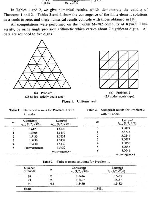
As $hown in Figure 1, 9i is di,vided into ,uniform mesh with equilateral .triangles
(10, 28, 91 nodes), so that Assumption 1 is satisfied. Also 92 is divided into uniform mesh
with right isosceles triangles (9, 25, 49, 81 nodes), so that Assumption 2 is,satisfied. The
numerical convergence criterion for the iteratign$ is employed, for example, in such a way
that
Alternating•Iterations of Finite Element Approximations 41
max '- '-- Åq10-b Uh .(Pi)-Uh .-i(Pi)
lsisN Uh .(Pi)
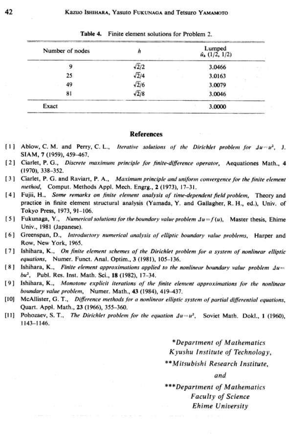
In Tables 1 and 2, we give numerical results, which demonstrate the validity of Theorems 1 and 2. Tables 3 and 4 show'the convergence of the finite element solutions as h tends to zero, and these numerical results coincide with those obtained in [8].
All computations were performed on the FAcoM M-382 computer at Kyushu Uni- versity, by using single precision arithmetic which carries about 7 significant digits. All
data are rounded to five digits.
(a) Probleml (b) Problem2
(28 nodes, strictly acute type) ' (25 nodes, acute type) Figurel. Uniformmesh.
Table l. Numerical results for Problem 1 with Table 2. Numerical results for Problem 2
91 nodes. with 81 nodes.
Lumped
Consistent Lumped
M uh,.(1/2, V'li7/6) ti,,.(112, ViiT/6) • M tih,.(1/2, 1/2)
O i.6120 1.6120 O 3.8029 -1 1.5408 l.5410 • 1 2.8777 2 1.5430 1.5433 2 3.0241 3 1.5430 l.5432 3 3.0017 4 1.5430 1.5432 4 3.oo50
5 (convergence) 1.5432 5 3.oo45
(convergence) 6 3.0046
--