Almost perfect quantum lattice action for low-energy SU(2) gluodynamics

Almost perfect quantum lattice action for low‑energy SU(2) gluodynamics

著者 Chernodub Maxim N., Fujimoto Shouji, Kato

Seikou, Murata Michika, Polikarpov Mikhail I., Suzuki Tsuneo

journal or

publication title

Physical Review D ‑ Particles, Fields, Gravitation and Cosmology

volume 62

number 9

page range 094506

year 2000‑10‑10

URL http://hdl.handle.net/2297/3474

Almost perfect quantum lattice action for low-energy SU „ 2 … gluodynamics

Maxim N. Chernodub,¹Shouji Fujimoto,² Seikou Kato,²Michika Murata,²Mikhail I. Polikarpov,¹and Tsuneo Suzuki²

1ITEP, B. Cheremushkinskaya 25, Moscow 117259, Russia

2Institute for Theoretical Physics, Kanazawa University, Kanazawa 920-1192, Japan 共Received 10 February 2000; published 10 October 2000兲

We study various representations of infrared effective theory of SU共2兲gluodynamics as a共quantum兲perfect lattice action. In particular we derive a monopole action and a string model of hadrons from SU共2兲gluody- namics. These are lattice actions which give almost cutoff independent physical quantities even on coarse lattices. The monopole action is determined by numerical simulations in the infrared region of SU共2兲gluody- namics. The string model of hadrons is derived from the monopole action by using BKT transformation. We illustrate the method and evaluate physical quantities such as the string tension and the mass of the lowest state of the glueball analytically using the string model of hadrons. It turns out that the classical results in the string model are near to the one in quantum SU共2兲gluodynamics.

PACS number共s兲: 12.38.Gc, 11.15.Ha

I. INTRODUCTION

The low-energy effective theory of QCD is important for an analytical understanding of hadron physics. Before the derivation of such an effective theory we have to explain the most important nonperturbative phenomenon, quark confine- ment. Wilson’s lattice formulation 关1兴 shows that confine- ment is a property of a non-Abelian gauge theory of strong interactions. At strong coupling the confinement is proved analytically. At weak coupling共near to the continuum limit兲 there are a lot of numerical calculations showing the confine- ment of color. The mechanism of confinement is, however, still not well understood. One of the approaches to the con- finement problem is to search for relevant dynamical vari- ables and to construct an effective theory in terms of these variables.

From this point of view the idea proposed by ’t Hooft关2兴 is very promising. It is based on the fact that after a partial gauge fixing共Abelian projection兲SU(N) gauge theory is re- duced to an Abelian U(1)^N⫺1 theory with N⫺1 different types of Abelian monopoles. Then the confinement of quarks can be explained as the dual Meissner effect which is due to condensation of these monopoles. The QCD vacuum is dual to the ordinary superconductor: the monopoles playing the role of the Cooper pairs. The confinement occurs due to the formation of a string with an electric flux between the quark and antiquark. It is a dual analogue of the Abrikosov string 关3兴. The mechanism of confinement is usually called the dual superconductor mechanism.

There are many ways to perform Abelian projection, but in the maximal Abelian 共MA兲 gauge 关4兴 many numerical results support the dual superconductor picture of confine- ment关5兴in the framework of lattice gluodynamics共see, for example, reviews关6,7兴兲. These results suggest that the Abe- lian monopoles which appear after the Abelian projection of QCD are relevant dynamical degrees of freedom in the in- frared共IR兲region. We expect hence, after integrating out all degrees of freedom other than the monopoles, an effective theory described by the monopoles works well in the IR region of gluodynamics.

The effective monopole action on the MA projection of

SU共2兲 lattice gluodynamics was obtained by Shiba and Su- zuki关8兴using an inverse Monte Carlo method关9兴. Assuming that the lattice action contains only quadratic terms of mono- pole currents, they found that the action has a form theoreti- cally predicted by Smit and van der Sijs 关10兴. This was the first derivation of an effective theory of lattice gluodynamics in terms of the monopole currents. However, the steps of block-spin transformation performed in Ref. 关8兴 were rather few to see the continuum limit. In Ref. 关11兴they considered also four- and six-point interactions assuming a direction symmetric action on the large (48⁴) lattice. More steps of the block-spin transformations were carried out also. It is stressed that the action seems to satisfy a scaling behavior, that is, it depends on the physical length b⫽na(␤^{) alone,} where n is the number of the blocking transformations and a(␤) is the lattice spacing. This remarkable scaling is con- sistent with the behavior of the perfect action on the renor- malized trajectory 共RT兲 which is an effective theory in the continuum limit formulated on the lattice with the lattice distance b. Here b plays a role of the physical scale at which the effective theory is considered. On RT, although we can predict physical quantities only on the b lattice sites, they are the same as evaluated from the continuum theory. For ex- ample, the continuum rotational invariance should be satis- fied. The restoration of the continuum rotational invariance for the quark-antiquark static potential was studied using a naive Wilson loop operator. However, the continuum rota- tional invariance was not confirmed in the IR region of SU共2兲gluodynamics关12兴. This is because the cutoff effect of such an operator is of order of the lattice spacing of the coarse lattice. To check restoration of the continuum rota- tional invariance, we should determine the correct form of physical operators 共the perfect operator兲as well as the per- fect action on the blocked lattice.

The main task of this publication is to derive the perfect monopole and the string action as a low-energy effective theory of SU共2兲gluodynamics and evaluate physical quanti- ties analytically using a renormalized operator. In Sec. II we discuss how to derive the renormalized monopole and the string action from SU共2兲 gluodynamics. We show new re- sults of the analysis of the monopole action which is ob-

tained by using inverse Monte Carlo method. In Sec. III we discuss how to construct the perfect operator for the static potential. In Sec. IV we calculate the string tension and the glueball mass for the SU共2兲 gluodynamics in terms of the strong coupling expansion of the string model analytically. It turns out that the classical results in the string model is near to the one in quantum SU共2兲gluodynamics. The continuum rotational invariance of the static potential is shown also ana- lytically. In Sec. V we analyze the numerical results in de- tails. Section VI is devoted to concluding remarks.

II. ALMOST PERFECT MONOPOLE ACTION FROM SU„2…GLUODYNAMICS

A. Our method

The method to derive the monopole action is the follow- ing.

共1兲 We generate SU共2兲 link fields 兵^U(s,␮⁾其 ^{using the} simple Wilson action for SU共2兲gluodynamics. We consider 24⁴ and 48⁴ hypercubic lattice for␤⫽2.0–2.8.

共2兲Next we perform an Abelian projection in the maxi- mal Abelian gauge to separate Abelian link variables 兵^u(s,␮⁾⫽e^i␪␮(s)其^(⫺␲⭐␪_␮^(s)⬍␲) from gauge fixed SU共2兲 link fields.

共3兲 Monopole currents can be defined from Abelian plaquette variables␪_␮␯(s) following DeGrand and Toussaint 关13兴. The Abelian plaquette variables are written by

␪_␮␯共s兲⬅␪_␮共s兲⫹␪_␯共s⫹␮^ˆ兲⫺␪_␮共s⫹␯^ˆ兲⫺␪_␯共s兲 关⫺4␲⬍␪␮␯共s兲⬍4␲兴. 共1兲 It is decomposed into two terms:

␪␮␯共s兲⬅^¯␪␮␯共s兲⫹2␲ⁿ␮␯共s兲, 关⫺␲⭐^¯␪␮␯共s兲⬍␲兴. 共2兲 Here, ^¯␪_␮␯(s) is interpreted as the electro-magnetic flux through the plaquette and the integer n_␮␯(s) corresponds to the number of Dirac string penetrating the plaquette. One can define quantized conserved monopole currents

k_␮共s兲⫽1

2⑀_␮␯␳␴⳵_␯ⁿ_␳␴共s⫹␮^ˆ兲, 共3兲 where ⳵ denotes the forward difference on the lattice. The monopole currents satisfy a conservation law⳵_␮

⬘

^k␮(s)⫽0 by definition, where⳵

⬘

denotes the backward difference on the lattice.

共4兲We consider a set of independent and local monopole interactions which are summed up over the whole lattice. We denote each operator asSi关k兴. Then the monopole action can be written as a linear combination of these operators

S关k兴⫽兺i

G_iSi关k兴, 共4兲 where G_i are coupling constants.

We determine the set of couplings G_ifrom the monopole current ensemble 兵^k␮(s)其 with the aid of an inverse Monte

Carlo method first developed by Swendsen and extended to closed monopole currents by Shiba and Suzuki 关8,9兴.

Practically, we have to restrict the number of interaction terms. It is natural to assume that monopoles which are far apart do not interact strongly and to consider only short- ranged interactions of monopoles. The form of actions adopted here is 27 quadratic interactions and four-point and six-point interactions. We have not assumed a direction sym- metric form of the action as done in Ref.关11兴. The detailed form of interactions are shown in Appendix A. Note that all possible types of interactions are not independent due to the conservation law of the monopole current. So we get rid of almost all the perpendicular interactions by the use of the conservation rule. The validity of the truncation has been studied and supported in the earlier works. For details, see Refs. 关8,11兴.

共5兲 We perform a block-spin transformation in terms of the monopole currents on the dual lattice to investigate the renormalization flow in the IR region. We adopt n

⫽1,2,3,4,6,8 extended conserved monopole currents as an n blocked operator 关14兴:

K_␮共s⁽ⁿ⁾兲⫽_{i, j,l}ⁿ兺^⫺_⫽¹₀ ^{k␮关ns(n)⫹共n⫺1兲␮ˆ⫹i␯ˆ⫹j␳ˆ⫹l␴ˆ兴}

共5兲

⬅Bk_␮共s⁽ⁿ⁾兲. 共6兲

The renormalized lattice spacing is b⫽na(␤) and the con- tinuum limit is taken as the limit n→⬁ for a fixed physical length b.

We determine the effective monopole action from the blocked monopole current ensemble 兵^K␮(s⁽ⁿ⁾)其^{. Then one} can obtain the renormalization flow in the coupling constant space.

共5兲The physical length b⫽na(␤) is taken in unit of the physical string tension冑␴phys. We evaluate the string tension

␴latfrom the monopole part of the Abelian Wilson loops for each␤ since the error bars are small in this case. The lattice spacing a(␤) is given by the relation a(␤⁾⫽冑␴lat/␴phys

关11兴. Note that b⫽1.0␴phys⫺1/2

corresponds to 0.45 fm, when we assume ␴phys⬵(440 MeV)².

B. Numerical results

We list new results below in comparison with earlier nu- merical analysis of the monopole action.

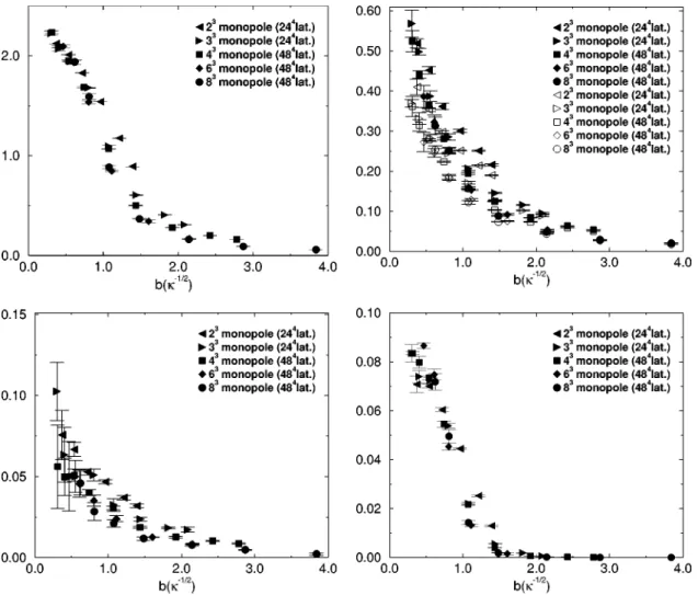
共1兲The inverse Monte Carlo method works well and the coupling constants of the action are fixed beautifully. The quadratic coupling constants and four-point coupling con- stant are plotted versus the physical length b⫽na(␤^{) for} each n extended monopole in Fig. 1. The first three figures show quadratic self coupling G₁(b), quadratic nearest- neighbor couplings 关G₂(b) 共black symbol兲, G₃(b) 共open symbol兲兴and G₁₀(b), respectively. The self-coupling term is dominant and the coupling constants decrease rapidly as the distance between the two monopole currents increases.

G₁共b兲ⰇG₂共b兲⬃G₃共b兲⬎•••⬎G₁₀共b兲⬎•••.

The four-point coupling constant becomes negligibly small in comparison with the quadratic couplings for large b region (b⬎1.5␴phys⫺1/2). The six-point coupling constant behaves similarly as the four-point coupling does and becomes much smaller for large b region:

quadratic couplingsⰇfour-point coupling Ⰷsix-point coupling.

From these figures we see a scaling of the action S关k_␮,n,a(␤⁾兴→S关K_␮,b⫽na(␤⁾兴 for fixed physical length b⫽na(␤) looks almost good for n⭓4. The obtained action appears to be a good approximation of the action on the RT.

共2兲 In Fig. 2 we plot the projected lines 关G₁(b)

⫺G₂(b), G₂(b)⫺G₃(b), and G₁(b)-4-point, respectively兴of the renormalization flow. Each flow line for smaller ␤ 共which corresponds to larger b) is beautifully straight with very small errors. The quadratic interactions for monopoles are dominant for larger b, that is, only the quadratic interac- tion subspace seems sufficient in the coupling space for low- energy SU共2兲 gluodynamics. We also see the effective monopole action tends to go to the weak coupling region when we go to the infrared region of SU共2兲gluodynamics.

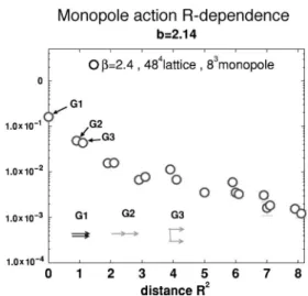
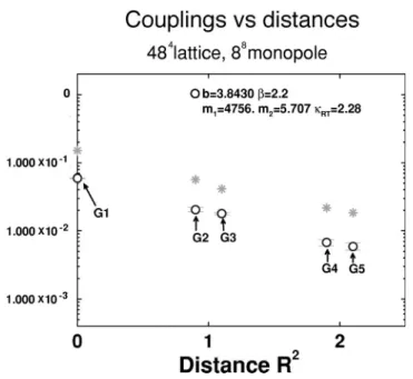
共3兲The quadratic coupling constants at b⫽2.14 are plot- ted versus the squared distance R²in unit of squared physical length b² in Fig. 3. We see the direction asymmetry of the current action.共For example, G₂⫽G₃.兲This behavior of the action does not occur in the case of compact QED, because the monopole action can be obtained from the Villain form of compact QED exactly in an analytical way and it does not depend on the direction between two monopole currents. In Ref.关11兴they have neglected this effect and have considered a direction symmetric form of the monopole action but as we will see later that this direction asymmetry of the current action is natural and important features of the perfect lattice action.

III. A PERFECT OPERATOR FOR PHYSICAL QUANTITIES

In previous sections we have studied the renormalized monopole actionS关k兴performing block spin transformation up to n⫽8 numerically, and have found the scaling for fixed physical length b looks almost good. If the continuum rota- tional invariance of physical observables is satisfied in addi- tion in the framework of S关k兴, we can regard S关k兴 as a good approximation of RT.

FIG. 1. The couplings of quadratic interaction term and 4-point interaction term versus physical length b.

A. Improved and perfect operator

In gluodynamics, the string tension from the static poten- tial is one of important physical quantities. However, it is a problem how to evaluate the static potential between electri- cally charged particles after Abelian projection. In the earlier work 关12兴 we considered a naive Abelian Wilson loop op- erator and S关k兴 on the coarse lattice to evaluate the static potential, but the continuum rotational invariance of the po- tential could not be well reproduced even for the infrared region of SU共2兲 gluodynamics. This is because the cutoff

effect of such an operator is of order of the lattice spacing of the coarse lattice. Only the scaling behavior of the action is insufficient. We should also adopt improved physical opera- tors on the coarse lattice in order to get the correct values of physical observables. An operator giving a cutoff indepen- dent value on RT is called the perfect operator.

B. The method

As will be shown in Sec. III D, when we consider a monopole action composed of general quadratic interactions FIG. 2. The renormalization flow on the projected plane.

alone, a block spin transformation can be done analytically 关15兴. We find a perfect operator for a static potential starting from an operator in the continuum limit. The continuum ro- tational invariance is shown exactly with the operator. This is an example of a perfect operator.

What happens in low-energy SU共2兲 gluodynamics? It is natural that one can not perform a block spin transformation analytically. However, as shown in the previous section, the Abelian monopole action S关k兴 which is obtained numeri- cally is well approximated by quadratic interactions alone for large b. The monopole action on the renormalized trajectory 共RT兲 is expected to be near to the quadratic coupling con- stant plane in the infrared region. We can perform the ana- lytic block spin transformation along the flow projected on the quadratic coupling constant plane as shown in Fig. 4.

When we define an operator on the fine a lattice, we can find a perfect operator along the projected flow in the a→0 limit for fixed b. Let us adopt the perfect operator on the projected space as an approximation of the correct operator for the actionS关k兴 on the coarse b lattice. It will be shown in the following Sec. III E that the above standpoint may be justi- fied as long as the quadratic monopole interactions are domi- nant.

C. Various operators for a static potential

There is another problem what is the correct operator for the Abelian static potential in Abelian projected SU共2兲gluo- dynamics on the fine a lattice. First let us consider the fol-

lowing Abelian gauge theory of the generalized Villain form on a fine lattice with a very small lattice distance:

S关␪^,n兴⫽ 1

4␲² _s,s⬘兺_;␮⬎␯ ^{关⳵[␮␪␯]共s兲⫹2␲n␮␯共s兲兴}

⫻共⌬LD₀兲共s⫺s

⬘

兲关⳵[␮␪_␯]共s

⬘

兲⫹2␲ⁿ_␮␯共s

⬘

兲兴, 共7兲 where ␪␮(s) is a compact Abelian gauge field and the integer-valued tensor n_␮␯(s) comes from the periodicity of the lattice action共7兲. Both of the variables are defined on the original lattice.⌬L(s⫺s

⬘

⁾⫽⫺⳵⳵

⬘

␦s,s⬘is the lattice Laplac- ian and we write D₀⫽␤⌬L⫺1⫹D₀

⬘

for later convenience, where D₀

⬘

is a general operator. Since we are considering a fine lattice near to the continuum limit, we assume the direc- tion symmetry of D₀

⬘

. Note that D₀⫽2␲²␤V⌬L⫺1 corre- sponds to the ordinary Villain action for compact QED. In this type of model, it is natural to use an Abelian Wilson loop W(C)⫽exp(i兺_C„␪_␮^(s),J_␮^(s)…) for particles with funda- mental Abelian charge, where J_␮(s) is an Abelian integer- charged electric current. The expectation value of W(C) is written as

具^W共C兲典⫽

冓

^exp

^再

^{i兺s,␮ J␮共s兲␪␮共s兲}

^冎 冔

^{⫽Z关J兴/Z关0兴, 共8兲}

Z关J兴⬅

冕

⫺␲

␲ 兿_s;␮ ^{d␪␮共s兲}_n␮␯(s)兺^⫹⬁_⫽⫺⬁ ^exp

再

^{⫺S关␪,n兴}

⫹i兺s,␮ J_␮共s兲␪_␮共s兲

冎

^{. 共9兲}

Next it is known that the theory with the above action共7兲 is equivalent to the lattice form of the modified London limit of the dual Abelian Higgs model关16兴as shown in Appendix B

S关C,␾^,l兴⫽ 1

4␤ s;兺␮⬎␯ 关⳵[␮C_␯]共s兲兴²⫹1

4 _s,s兺_⬘;␮ ^{关⳵␮␾共s兲}

⫺C_␮共s兲⫹2␲^l␮共s兲兴D₀

⬘

^⫺1共s⫺s

⬘

兲关⳵␮␾共s

⬘

兲

⫺C_␮共s

⬘

兲⫹2␲^l␮共s

⬘

兲兴. 共10兲 The static potential for electrically charged particles is evalu- ated by a dual ’t Hooft operator

H共C兲⫽exp

再

^{⫺41␤ s;␮⬎␯兺 关⳵[␮C␯]共s兲⫺2␲*S␮␯J 共s兲兴2}

⫹ 1

4␤ _s;兺_␮⬎␯ ^{关⳵[␮C␯]共s兲兴2}

冎

^{, 共11兲}

where *S_␮␯^J (s) is dual to the surface which is spanned inside the contour J_␮(s).

Thirdly, when use is made of the Beresinskii-Kosterlitz- Thouless 共BKT兲 transformation 关17–19兴, the action 共7兲 is equivalent to the following monopole action:

FIG. 3. The distance dependence of the couplings of quadratic interaction terms at b⫽2.14.

FIG. 4. Flow of the couplings under block spin transformations.

S关k_␮共s兲兴⫽_s,s兺_⬘,␮ ^{k␮共s兲D0共s⫺s}

^⬘

^兲k␮共s

^⬘

^{兲. 共12兲}

We see that the area law term is given correctly also by the following operator in the monopole representation as shown in Appendix B:

W_m共C兲⫽exp

冉

^{2␲i兺s,␮ N␮共s兲k␮共s兲}

冊

^{, 共13兲}

N_␮共s兲⫽兺_s⬘ ^{⌬L⫺1共s⫺s}

^⬘

^兲

⫻1

2⑀_␮␣␤␥⳵_␣^S_␤␥^J 共s

⬘

⫹␮^ˆ兲, 共14兲

where S_␤␥^J (s

⬘

^⫹␮ˆ ) is a plaquette variable satisfying

⳵_␤

⬘

^S_␤␥^{J (s)}⫽J_␥(s) and the coordinate displacement␮^{ˆ is due} to the interaction between dual variables.

However, the expectation values of the above three opera- tors are not completely equivalent. When we consider infra- red effective Abelian theories, it is natural that the static potential between electric charges becomes Coulombic in the deconfinement phase. The ’t Hooft operator in the dual Abe- lian Higgs model or the Wilson loop in the generalized Vil- lain form reproduce this behavior. However, it is stressed that all three operators give the same area law, since the differences give only Coulombic or Yukawa potentials.

Since we are interested in the string tension, let us consider the operator共13兲from now on. See Appendix B for details.

D. Analytic block spin transformation

We construct a block spin transformation共6兲of monopole currents.¹ Integrating out the monopole current variable on the fine lattice we arrive at an effective action and the loop operator for the static potential on the coarse lattice关15兴. Let us start from

具^Wm共C兲典^⫽_k␮(s)兺_⫽⫺⬁

⳵_␮⬘^k␮(s)⫽0

⬁

exp

再

^{⫺s,s兺⬘,␮k␮共s兲D0共s⫺s}

^⬘

^兲k␮共s

^⬘

^兲

⫹2␲ⁱ兺s,␮ N_␮共s兲k_␮共s兲

冎

⫻_s兿(n),␮ ␦关K_␮共s⁽ⁿ⁾兲⫺Bk_␮共s⁽ⁿ⁾兲兴/Z关k兴. 共15兲

The cutoff effect of the operator共15兲is O(a) by definition.

This␦-function renormalization group transformation can be done analytically. Taking the continuum limit a→0, n→⬁

共with b⫽na is fixed兲finally, we obtain the expectation value of the operator on the coarse lattice with spacing b⫽na 关15兴:

具^Wm共C兲典⫽exp

再

^⫺␲2

^冕

^{⫺⬁⬁ d4xd4y兺␮ N␮共x兲}

⫻D₀^⫺1共x⫺y兲N_␮共y兲⫹␲^2b8 兺

s⁽ⁿ⁾,s⁽ⁿ⁾⬘

␮,␯

B_␮共bs⁽ⁿ⁾兲

⫻D_␮␯共bs⁽ⁿ⁾⫺bs^(n)⬘兲B_␯共bs^(n)⬘兲

冎

⫻_b3K_␮(bs)兺⫽⫺⬁

⳵_␮⬘^K␮⫽0

⬁

exp

再

^{⫺S关K␮共s(n)兲兴}

⫹2␲^ib8 兺

s⁽ⁿ⁾,s⁽ⁿ⁾⬘

␮,␯

B_␮共bs⁽ⁿ⁾兲D_␮␯共bs⁽ⁿ⁾⫺bs^(n)⬘兲

⫻K_␯共bs^(n)⬘兲

冎 ^冒

^b3K_⳵^␮_␮⬘^(bs)兺K_␮⫽^⫽⫺⬁0

⬁

Z关K,0兴, 共16兲

where

B_␮共bs⁽ⁿ⁾兲⬅lim

a→0 n→⬁

a⁸_s,s兺_⬘,␯ ^{⌸¬␮共bs(n)⫺as兲}

⫻

再

^{␦␮␯⫺兺␳⳵␮⳵⳵␳␯}

^⬘

^⳵␳

^⬘ 冎

⫻D₀^⫺1共as⫺as

⬘

兲N_␯共as

⬘

兲, 共17兲

⌸_¬␮共bsⁿ⫺as兲⬅ 1

n³␦关nas_␮⁽ⁿ⁾⫹共n⫺1兲a⫺as_␮兴

⫻_i(兿_⫽␮)

冉

^{nI兺⫽⫺01 ␦共nasi(n)⫹Ia⫺asi兲}

冊

^.

共18兲 S关K_␮(s⁽ⁿ⁾)兴 denotes the effective action defined on the coarse lattice

S关K_␮共s⁽ⁿ⁾兲兴⫽b⁸ 兺

s⁽ⁿ⁾,s⁽ⁿ⁾⬘ 兺_␮,␯ ^{K␮共bs(n)兲}

⫻D_␮␯共bs⁽ⁿ⁾⫺bs^(n)⬘兲K_␯共bs^(n)⬘兲. 共19兲

1Note that the current K_␮(s⁽ⁿ⁾) on the coarser lattice with a lattice distance b⫽na satisfies the current conservation⳵_␮⬘^K_␮^(s(n))⫽0 by definition.

Since we take the continuum limit analytically, the operator共16兲does not have any cutoff effect.

The momentum representation of D_␮␯(bs⁽ⁿ⁾⫺bs^(n)⬘) takes the form

D_␮␯共p兲⫽A_␮␯^GF⫺1共p兲⫺1

␭ pˆ_␮pˆ_␯

共pˆ²兲²e^{i( p␮⫺p␯)/2}, 共20兲

where A_␮␯

⬘

^GF⫺1( p) is the gauge-fixed inverse of the following operator:

A_␮␯

⬘

共p兲⬅

冉

^{i兿⫽41 li⫽⫺⬁兺⬁}

冊 再

^{D0⫺1共p⫹2␲l兲}

冋

^{␦␮␯⫺共p⫹兺2i␲共lp兲␮⫹共p2⫹␲l2兲␲i2l兲␯}

册

^{共p⫹兿2i␲共lp兲␮⫹共p2⫹␲l2兲␲i2 l兲␯}

冎 ^冉

^{兿i⫽pˆ41␮pˆpˆ␯i}

^冊

^{2. 共21兲}

The explicit form of D_␮␯( p) is written in Ref.关15兴. Perform- ing the BKT transformation explained in Appendix B on the coarse lattice, we can get the loop operator for the static potential in the framework of the string model:

具^Wm共C兲典⫽具^Wm共C兲典cl

⫻1

Z _␴␮␯(s)兺_⫽⫺⬁

⳵[␣␴_␮␯](s)⫽0

⬁

exp

再

^{⫺␲2␮⫽␣␯⫽␤兺s,s⬘ ␴␮␣共s兲⳵␣⳵␤}

^⬘

⫻D_␮␯^⫺1共s⫺s₁兲⌬L⫺2

共s₁⫺s

⬘

兲␴␯␤共s

⬘

兲

⫺2␲²_s,s兺_⬘

␮,␯

␴␮␯共s兲⳵␮⌬L⫺1共s⫺s

⬘

兲B_␯共s

⬘

兲

冎

^{. 共22兲}

具^Wm(C)典cl is defined by

具^Wm共C兲典cl⫽exp

再

^⫺␲2

^冕

^{⫺⬁⬁ d4x d4y兺␮ N␮共x兲‘}

⫻D₀^⫺1共x⫺y兲N_␮共y兲

冎

^{. 共23兲}

E. The on-axis case

In the above calculation, we have introduced the source term corresponding to the loop operator for the static poten- tial on the fine a lattice and have constructed the operator on the coarse b lattice by making the blockspin transformation.

To check the validity of our analysis, it is to be emphasized that the same string tension for the flat on-axis Wilson loop can be obtained for I,T→⬁ when we consider a naive Wil- son loop operator on the coarse b lattice instead of that on the fine lattice共13兲. When we consider only quadratic inter- actions for the monopole action, we get the classical string tension from the large flat Wilson loop as follows关15兴:

␴L⫽

冕

⫺␲

␲ d²p

共2␲兲²⌬L⫺2共k₁,k₂,0,0兲

冋

^{sin2k22D⫺1共k1,k2,0,0;1ˆ兲}

⫹sin²k₁

2 D^⫺1共k₁,k₂,0,0;2ˆ兲

册

^{, 共24兲}

where D denotes the coupling of the monopole action deter- mined numerically on the coarse b lattice. For I→⬁ and T

→⬁, we can easily show that ␴L agrees exactly with the string tension derived later from Eq. 共23兲 关15兴. Therefore, our analysis is natural as long as the quadratic monopole action is a good approximation in the IR region of SU共2兲 gluodynamics. Note that we can show both quantum fluctua- tion parts also coincide.

IV. ANALYTICAL RESULTS OF SU„2…GLUODYNAMICS A. Parameter fitting

As shown already, the 共numerically obtained兲 effective monopole action for SU共2兲gluodynamics in the IR region is well dominated by quadratic interactions. Hence we regard the renormalization flow obtained in Sec. III D as a projec- tion of RT to the quadratic-interaction plane as written in Fig. 4. We adopt the perfect operator discussed in the previ- ous section as the correct one on the coarse b lattice in the low-energy SU共2兲 gluodynamics. In order to know the ex- plicit form of the operator, we need first to fix D₀(s⫺s

⬘

^).

This can be done by comparing D_␮␯(bs⁽ⁿ⁾⫺bs^(n)⬘) with the set of numerically obtained coupling constants of the mono- pole action 兵^Gi(b)其 in Sec. II.

We assume D₀(s⫺s

⬘

) in the monopole action 共12兲 to take ␣^¯␦s,s⬘⫹␤^¯⌬L⫺1(s⫺s

⬘

⁾⫹␥^¯⌬L(s⫺s

⬘

^{), where}␣^{¯ ,} ␤^{¯ , and}

␥

¯ are free parameters. We can consider more general qua- dratic interactions, but as we see later, this choice is suffi- cient to derive the IR region of SU共2兲gluodynamics.

The inverse operator of D₀( p)⫽␣^¯⫹␤^{¯ /p2}⫹␥^{¯ p2takes the} form

D₀^⫺1共p兲⫽␬

冉

^{p2m⫹12m12⫺p2m⫹22m22}

冊

^{, 共25兲}

where the new parameters ␬^{, m}1, and m₂ satisfy ␬^(m1 2

⫺m₂²)⫽␥^¯⫺1,m1

2⫹m₂²⫽␣^{¯ /}␥^{¯ ,m}1

2m₂²⫽␤^{¯ /}␥¯ . Substituting Eq.

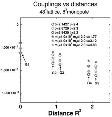
共25兲 into Eq.共21兲 and performing a First Fourier transform 共FFT兲on the 16⁴ lattice for the several input values ␬^{, m}1, and m₂ we calculate D_␮␯( p). Then one can obtain distance dependence of the D_␮␯(bs⁽ⁿ⁾⫺bs^(n)⬘). By matching the dis- tance dependence of the D_␮␯(bs⁽ⁿ⁾⫺bs^(n)⬘) with numerical ones, one can fit the free parameters␬^{, m}1, and m₂. We find that the ratio m₁/m₂ is around 10⁴, but m₁ and m₂cannot be fixed well separately. Their optimal values for b⫽2.1, 2.9, and 3.8 are given in Table I, where we fix m₁⫽1.0⫻10⁴and m₂⫽12 for all b. The coupling constants with the optimal values are illustrated in Fig. 5. Note that, in this figure, the lattice monopole action obtained from the continuum by ana- lytical blocking also show the direction asymmetry.

B. The string tension

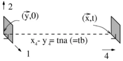
Let us evaluate the string tension using the perfect opera- tor共22兲. The plaquette variable S_␣␤^J in Eq.共14兲for the static potential V(Ib,0,0) is expressed by

S_␣␤^J 共z兲⫽␦␣1␦␤4␦共z₂兲␦共z₃兲␪共z₁兲␪共Ib⫺z₁兲

⫻␪共z₄兲␪共Tb⫺z₄兲. 共26兲 In Sec. II B we have seen that the monopole action on the dual lattice is in the weak coupling region for large b. Then the string model on the original lattice is in the strong cou- pling region. Therefore, we evaluate Eq. 共22兲by the strong coupling expansion. The method can be shown diagrammati- cally in Fig. 6.

1. The classical part

As explicitly evaluated in Ref. 关15兴, the classical part of the string tension coming from Eq.共23兲is

␴cl⫽␲␬

2 lnm₁

m₂. 共27兲

冑␴cl/␴phys using the optimal values ␬^{, m}1, and m₂ are given in Table II, where ␴physis the physical string tension.

The scaling of冑␴cl/␴physfor physical length b seems good, although its absolute value is larger than 1. The difference will be analyzed later in Sec. V.

2. Quantum fluctuations

The next to leading quantum fluctuation term comes from the second part of Eq. 共22兲. It corresponds to the second figure in Fig. 6 and becomes关15兴

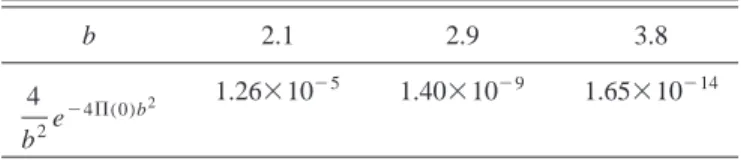
␴q f⫽⫺ 4

b²e^⫺4⌸(0)b2, 共28兲 where⌸(0) is the self-coupling constant of the string action 共22兲. The total string tension is the sum␴tot⫽␴cl⫹␴q f.

The quantum corrections for the string tension are given in Table III. We see they are negligibly small in IR region of SU共2兲 gluodynamics. We can evaluate physical quantities using the classical part alone in the strong coupling expan- sion of the string model. Therefore, the strong coupling ex- pansion works good and it is found that the classical string tension in the string model is near to the one in quantum SU共2兲gluodynamics.

TABLE II. 冑␴cl/␴physfor b⫽2.1, 2.9, and 3.8.

b 2.1 2.9 3.8

冑␴^␴phys^cl

1.64 1.56 1.45

TABLE I. The optimal values␬, m₁, and m₂ for b⫽2.1, 2.9, and 3.8 from the inverse Monte Carlo method.

b 2.1 2.9 3.8

␬ 1.76 3.12 4.83

m₁ 1.0⫻10⁴ 1.0⫻10⁴ 1.0⫻10⁴

m₂ 12.0 12.0 12.0

FIG. 5. The coupling constants with the optimal values␬, m1, and m₂for b⫽2.1, 2.9, and 3.8 from the comparison with numeri- cal data.

FIG. 6. The strong coupling expansion of the Wilson loop cal- culation.