yvF.fl r11,44 r,,,:r

(1)

Master's Thesis

Design and Evaluation of a

Method to Enhance Robustness of MCMC-Based Autonomous

Decentralized Mechanism for VM Assignment Problem

14892532 Masaya YOKOTA

Supervisor Prof. Masaki AI DA

January, 2016

Division of Management System Engineering

Graduate School of System Design Tokyo Metropolitan University

(2)

(3)

—i—

Contents

Chapter 1 1.1 1.2

Introduction

Background ...

Objective ...

1 1 4 Chapter 2

2.1 2.2 2.3

The MCMC-Based Autonomous Decentralized Mechanism System Model ...

Autonomous Node Action ...

Global property ...

5 5 7 8 Chapter 3

3.1 3.2

A Method for Enhancing Robustness of the MCMC-Based ADM 14 The Proposed Method ...14

Mechanism absorbing the impact of Environmental Fluctuation ... 15 Chapter 4

4.1 4.2 4.3 4.4

Simulation Experiment

Experiment Model ...

Characteristic of the Proposed Method ...

Regarding fluctuation in Traffic Rate ...

Regarding fluctuation of the Number of VM ...

18 . .18 . .20 . .24 . .31

Chapter 5 Conclusion 36

Acknowledgement 37

Bibliography 38

Appendix A A.1 A.2

MCMC property41

The Iimit of simple Monte Carlo ...41 Convergence of MCMC ...42

Appendix B B.1

Source Code45

Simulation Experiment for VM Assignment Problem ...45

(4)

— iii —

List of Figures

1.1 1.2

The image of VM assignment ...

VM concentrated assignment vs VM load decentralized assignment ...

3 3 2.1

2.2

3.1

An example of the system model with n = 7 and N = 4 ...

A relation image between P(M) and nodes assignmed in resources ...

Distribution P(M) and G(M) vs. Normalized distribution P(M) and G(M) . . . 6 9 16 4.1

4.2 4.3 4.4 4.5 4.6 4.7 4.8 4.9 4.10 4.11

4.12 4.13 4.14 4.15

4.16 4.17 4.18 4.19 4.20 4.21 4.22

DCN topology ...19

Probability density function P(M) in the previous method ...21

Probability density function P(M) in the proposed method ...21

System performance variable M in the previous method ...21

System performance variable M in the proposed method ...21

Percentage of VM assigned in each PM in the previous method ...22

Percentage of VM assigned in each PM in the proposed method ...22

Coefficient of variation CV[p] in the previous method ...22

Coefficient of variation CV[p] in the proposed method ...22

Coefficient of variation CV[p] vs. M using the proposed method and previous method ...23

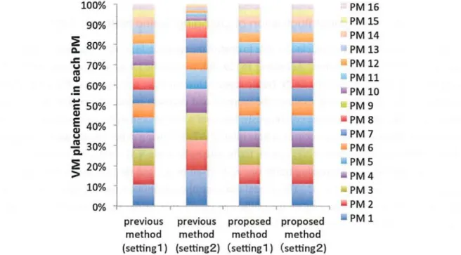
Percentage of VM assigned in each PM using traffic settings 1 and 2 in the proposed method and previous method ...25

Coefficient of variation CV[•] in traffic rate settings 1 and 2 in the previous method 25 Coefficient of variation CV [p] in traffic rate settings 1 and 2 in the proposed method 25 Coefficient of variation CV[p] in fluctuation of changing traffic rate in the proposed method and previous method ...28

Coefficient of variation CV [p] in fluctuation (AT,. = 1, Kr = 0.1) of changing traffic rate for different values of control parameter K in the proposed method . 28 Coefficient of variation CV[p] in fluctuation (ATr = 1, Kr = 0.1) in the proposed method ...28

Probability density function of CV [p] in fluctuation (AT,. = 1, Kr = 0.001) . . . 29

Probability density function of CV[p] in fluctuation (ATr = 0.1, Kr = 0.001) . . 29

Probability density function of CV[•] in fluctuation (AT,. = 0.01, Kr = 0.001) . . 29

Probability density function of CV[p] in fluctuation (ATr = 1, Kr = 0.1) ...29

Probability density function of CV[p] in fluctuation (ATr = 0.1, K,. = 0.1) . . . . 29

Probability density function of CV[p] in fluctuation (AT,. = 0.01, K,. = 0.1) . . . 29

(5)

— iv — List of Figures

4.23

4.24

4.25

4.26

4.27

4.28 4.29 4.30 4.31 4.32 A.1

Coefficient of variation CV[p] vs. M using the proposed method and previous method in traffic rate setting 2 ...

Coefficient of variation CV[p] for different values of parameter ,1 in the previous method ...

Coefficient of variation CV [p] for different values of parameter K in the proposed method ...

Coefficient of variation CV[p] in fluctuation of changing traffic rate in the proposed method and previous method ...

Coefficient of variation CV[p] in fluctuation (AT„ = 100, An = 1) of changing traffic rate for different values of control parameter K in the proposed method . oefficient of variation CV[p] in fluctuation (AT„ = 100, An = 1) in the proposed method ...

Probability density function of CV[p] in fluctuation (AT„ = 100, An = 1) . . . . Probability density function of CV[p] in fluctuation (AT„ = 100, An = 10) . . . Probability density function of CV [p] in fluctuation (AT„ = 200, An = 10) . . . Probability density function of CV[p] in fluctuation (AT„ = 300, An = 10) . . . The image of probability ...

30

31

34

34 35 35 35 35 42

(6)

1

Chapter 1

Introduction

1.1 Background

In recent years, progress of Information and Communications Technology (ICT) systems is remarkable [1]. Many people use not only a cell phone or a personal computer but also a smart- phone or a tablet terminal, and the frequency of use is increasing. ICT, including the Internet and cell phones, has prevailed on a global scale, and the Internet diffusion rate in the world is over 89.5% in 2012 [1]. In addition, the use of it spreads over various kind of industry, such as finance, medical, education, and so on. For instance, in a field of education, Ministry of Internal Affairs and Communications promotes using ICT, and many companies are providing educational services using it. Hence, ICT is deepening ties with society. In the field of business, driving the term "Big Data", is still fresh in our minds. Big Data is a broad term for data sets so large or com- plex that traditional data processing applications are inadequate. This term shows the fact that the amount of data we can use is becoming tremendous nowadays, and a technology to process it is also advanced. For example, in order to process of such numerous data, large-scale distributed processing technique such as Apache Haddop [2] has been made practical.

At the same time ICT increase, the mobile data traffic is also increasing. Cisco Systems, Inc.

showed grobal mobile data traffic forecast, 2014 to 2019 [3]. According to them, overall mobile data traffic is expected to grow to 24.3 exabytes per month by 2019, nearly a tenfold increase over 2014.

To accommodate such numerous traffic requests, many ICT systems are supported by large- scale and wide-area data centers. For instance, Google has distributed a large number of servers composed of its data center around the world [4], and many ICT systems provide service by using Google data center. In recent years, as represented by Cloud Computing, services via the data center is becoming more common, and it is expected such a data center is becoming larger and larger in order to improve computational capability and system reliability. And in order to handle sustainably large-scale and wide-area systems represented a data center, we need to realize a scalable control scheme. Hence, a scalable control scheme should be realized to handle

(7)

2 Chapter 1 Introduction

sustainably large-scale and wide-area systems like data centers.

In general, system control architecture is roughly categorized as Centralized Control (CC) or Autonomous Decentralized Control (ADC). Consider the situation that a system is composed of numerous nodes distributed in a wide area. In a CC, there is a management node and it has to gather state information of numerous nodes from the entire system, and controls intensively the state of all the nodes in the system. Hence, CC requires a large amount of time to gather state information in the large-scale and wide-area system, and cannot handle such a system against dynamic environment fluctuation. In an ADC, each node autonomously controls its own state on the basis of local information that can be gathered directly by the node. The local information is, in other words, the state information of neighboring nodes. Since each node uses only local information, ADC can quickly react for an environmental fluctuation. Hence, ADC is being actively discussed in order to build a scalable control scheme for large-scale and wide-area systems (see, e.g., [5-19]). In ADC, an autonomous node action influences a state of the system. Therefore such an action following an Autonomous Decentralized Mechanism (ADM) should be designed to be able to tie to the control of the entire system [5].

1.1.1 VM Assignment Problem

Recently cloud computing services have been activated [20]. For instance, some services (such as Amazon EC2 [21] and Microsoft Azure [22]) provide an extension of the computational resources by running a Virtual Machine (VM) in the cloud space, and they urged the release from an on-premises constraints. VM is an emulation of a particular computer system. VMs operate based on the computer architecture and functions of a real or hypothetical computer, and they enable to implement common operations which do not depend on differences in hardwares, and to share resources in multiple Physical Machines (PMs). By dividing the tasks for each process, we can realize distributed processing by VMs assigned in PMs. However, when using VM in Data Center Network (DCN) composed by PM, we should consider about some issue about a performance such as processing efficiency, energy efficiency, load balance, and so on [23].

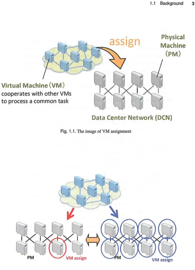
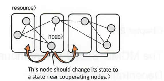
In DCN, there is a problem, called VM Assignment Problem [24]. How to assign VMs in the DCN is one of the significant issue to improve overall system performance and use resources effec- tively [25]. Figure 1.1 shows the image of VM assignment. Assuming that VMs are cooperating with other VMs to process a common task, and assigned a DCN composed PMs. In this situation, we can assume two opposite way to VM assignment. Considering efficient process, VMs having high traffic rate should be assigned in same or near PMs. On the other hand, Considering load decentralizing for a system, VMs should be assigned in entire PMs evenly 1.2. Significant point here is that we have to consider about these trade-off relationship in VM Assignment Problem. To build a scalable control scheme for this kind of situation, previous research about ADM based on Markov chain Monte Carlo (MCMC) is discussed.

(8)

1.1 Background 3

tiz e f \ = t:r

4.../...,14,.. ,

Virtual Machine (VM)

cooperates with other VMs to process a common task

assign _Machine^Physical

(PM)

507

Data Center Network (DCN)

Fig. 1.1. The image of VM assignment

[1-><13

PM

A/ _.

) .'i '----

yvF.fl r11,44 r,,,:r

... ,..._11 1

M a assignr0-, zfr,j,

am ,_1;

~

VM assign

Fig. 1.2. VM concentrated assignment vs VM load decentralized assignment

(9)

4 Chapter 1 Introduction

1.2 Objective

This paper discusses about MCMC-Based Autonomous Decentralized Mechanism (ADM).

MCMC (Markov Chain Monte Carlo) [26,27] is a method to generate a Markov process following a desired probability distribution of a statistical-mechanical variable (e.g., energy). Considering fluctuatuions, controling system state by using a probability distribution is better than the way of fixing in one optimized state. Because using a probability distribution can deal with fluctuatuions flexibly.

In [16], on the basis of MCMC, the authors designed an autonomous node action to control for the probability distribution of system performance variable that is an amount to quantify of a system state. In addition, they applied the method for solving the VM assignment problem.

In [17], the authors have proposed an advanced function of the MCMC-Based ADM as the so- lution for the VM assignment problem against simple environmental fluctuations. However they have not fully shown for its robustness against several environmental fluctuations. There are various kinds of environmental fluctuations for actual systems, so it is crucial to discuss robustness of the MCMC-Based ADM and improve its robustness if necessary.

This paper proposes a method of MCMC-Based ADM to enhance its robustness against severe environmental fluctuations. In the proposed method, each node autonomously adjusts its control parameter of the MCMC-Based ADM. Then, similarly to [16], this paper applies the proposed method to the VM assignment problem in DCN. Through simulation experiment, this paper clarifies that the effectiveness of the proposed method for severe environmental fluctuation . In addition, this paper evaluates the proposed mathod by comparing with the previous method [17], and try to get the new knowledge about MCMC-Base ADM.

This paper is organized as follows. Chapter 2 introduces MCMC-Based ADM [16]. Chapter 3 discusses the impact of environmental fluctuation on the MCMC-Based ADM, and designs an its adjustment method to absorb environmental fluctuations. Chapter 4 shows the fundamental property of the proposed method of MCMC-Based ADM, and the experiments conducted for investigating the robustness of the proposed method in data center networks. Finally, chapter 5 concludes this paper.

(10)

5

Chapter 2

The MCMC-Based Autonomous Decentralized Mechanism

The method, that connects the node action and the entire system state, is inspired by knowledge of statistical mechanics. Statistical mechanics provides a framework for relating the microscopic properties of individual atoms and molecules to the macroscopic properties of materials that can be observed in everyday life. Therefore, by using the mechanism of statistical mechanics, it is possible to tie the microscopic behavior such as node actions to the macroscopic behavior like a system state.

This chapter explains the MCMC-Based ADM [16] and its property, concrete mechanism, in other words, why an autonomous node action generate the desired probability distribution of system performance variable that is an amount to quantify of a system state.

2.1 System Model

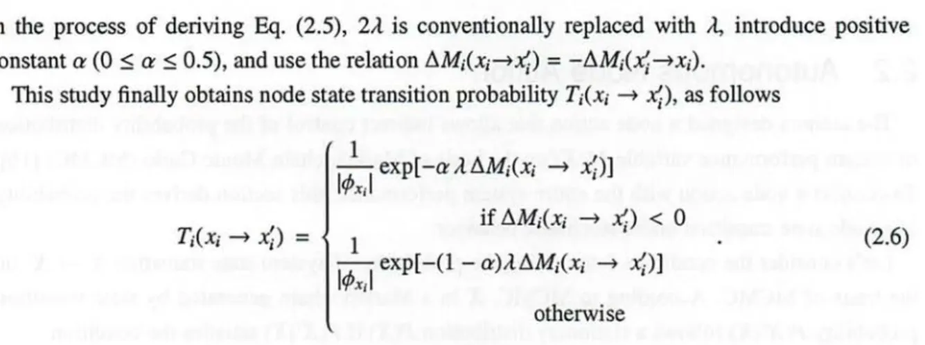
This subsection first introduces a system model in this thesis. Consider a distributed system in which n nodes interact with each other in order to process tasks. To process tasks, each node uses N distributed computational resources. The state of a node is determined by which resource is used in N resources. Fig. 2.1 shows an example of the system model with n = 7 and N = 4. In this figure, interacting nodes are represented by links. Each node prefers to use the same resource or near resources with frequently interacting nodes, so nodes would be concentrated to a few resources. However, for efficient task processing, the load decentralization among resources should be realized. Since there is a trade-off between the node concentration and the load decentralization, the system should adequately adjust the balance of them subject to the trade-off.

Let xi be node i's state that is the ID of the resource used by node i (xi E 1, .., N). Let us define system state X by combination (xi, ..., x„) of all node states. System state X influences the node concentration and the load decentralization, so we can assume that performance of the

(11)

6 Chapter 2 The MCMC-Based Autonomous Decentralized Mechanism

resource>

node>

This node should change its state to a state near cooperating nodes.>

Fig. 2.1. An example of the system model with n = 7 and N = 4

system depends on system state X. In addition, each resource has adjacency relationships with other resources. Let cbk be the set of resources that have an adjacency relationshipwith resource k.

Each node is permitted to move to one of the other resources that have the adjacency relationship Then, let us define system performance variable M(X) as

M(X) = rij d(xi, xj), 1=1 _EX;

(2.1) where xi is the set of nodes interacting with node i, rijis the interaction frequency between nodes i and j, and d(k, 1) is distance between resources k and 1. Let us assume rii = 0 and r13 = r31, d(xi, x3) = d(xj, xi). These are valuse given by information of the external environment.

Small M(X) means strong node concentration but weak load decentralization. For example, if nodes i and j are assigned to a same resource (i.e., xi = xj), they are most strongly interacting . However, if all nodes are assigned to a same resource, M(X) becomes minimum value , load of the assigned resource is terrible. Hence, M(X) should be controlled by considering the strengths of node concentration and node decentralization, in other words, by controlling M(X), the system adequately adjusts the balance of them.

Node i indirectly controls the probability distribution of system performance variable M by ap- propriately changing its state xi. To change node state xi, node i should use only local information for node j E Xi in ADM.

(12)

2.2 Autonomous Node Action 7

2.2 Autonomous Node Action

The authors designed a node action that allows indirect control of the probability distribution of system performance variable M(X) on the basis of Markov chain Monte Carlo (MCMC) [16].

To connect a node action with the entire system performance, this section derives the probability of a node state transition under stochastic behavior.

Let's consider the condition determining the probability of system state transition X X' on the basis of MCMC. According to MCMC, X in a Markov chain generated by state transition probability P(X'IX) follows a stationary distribution P(X) if P(X'IX) satisfies the condition

P(X'IX) P(X) = P(XIX') P(X'),(2.2)

and the ergodic condition, that is, the probability happening any states after some state transition is larger than 0.

Next, derive probability Ti(xi-'4) of node i' s state transition xi -> xl according to the condition (2.2). let us give X' = (xl, ..., x'), and the stationary distribution P(X) by exponential form (i.e., P(X) = Ae-AM(x) where A > 0). To focus on only the node i, we regard the states as

xi and xi = xJ. By using P(X) = Ae-'i'(X), Eq. (2.2) is rewritten by

P(Y'IY

P(XIX'). [.

Ti(xi->x)

Tl(x,-> x)= expE nj [d(x;, xJ) - d(xi, xi)]

To use the amount of change of M(X) with respect to the state transition of node i given by

AMi(xi-'xl) = ri J [d(x;, x3) - d(xi, xi)] ,

J EXi

the equation (2.3) is denoted by Ti(xi->x')

--- = exp [-A.AMi(xi -> x;)]

Ti(xi—xi)

exp [-a1LMi(xi -> 4)]

exp [-(l - a)AAMi(xi -> xa )]

I I exp [-aAAMi(xi -* xl )]

I~,lexp [-(1 - a)Ai Mi(xi—x'i)]•

(2.3)

(2.4)

(2.5)

(13)

In the process of deriving Eq. (2.5), 2/1 is conventionally replaced with A, introduce positive constant a (0 < a < 0.5), and use the relation L\Mi(xi—'x;) = —OMi(x;—)xi).

This study finally obtains node state transition probability Ti(xi —) x;), as follows

Ti(xi -) .4) = 1 kfrx; I

1 (Oxi I

exp[-rA.AMi(x, -) x;)]

if OM;(xl -) xii) < 0 exp[-(1 - cr)AiM;(xi -) xi)]

otherwise

(2.6)

Each node is assumed to use a common value among all nodes as the value of A. By using

Eq. (2.6), each node can change its state autonomously because T;(xi -) x;) depends on OM;(x; -*

x;) instead of M. T;(xi -) xi) for a = 0 is the same as the state transition probability used in the M-H algorithm [26]. To satisfiy the ergodic condition, all states have to be connected in the state transition graph.

If each node uses state transition probability T i(x; —) xx) by Eq. (2.6), system performance variable M follows the probability distribution

P(M) = Z G(M) exp(-AM) _1 G(M)eAM,(2.7) YEnM G(Y) exp(-AY) Z

where G(Y) is the system state density distribution, which is the number of system state if the system performance variable is equal to Y, and S2M is the set of all possible values of system performance variable M. According to Eq. (2.7), if A = 0, P(M) is proportional to G(M). In this case, the MCMC-based ADM is equivalent to the control where each node selects its state at random. In addition, as control parameter A. increases, each node controls its state to lead to the emergence of smaller M. Therefore, the MCMC-based ADM can adjust M(X) by changing A..

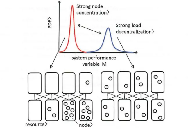
Fig. 2.2 shows a relation image between P(M) and node assigned in resources. In this figure, red line means strong node concentration but weak load decentralization and blue line means week node concentration but strong load decentralization. In addition, lower figure shows resources and node distribution. This probability distribution reflects system state, hence turning P(M) is realized by changing A. and it correspond with system state.

2.3 Global property

2.3.1 The Time for becoming a Steady State

The indirect control of M by using Eq. (2.6) is achieved when the system state becomes steady state where M follows the probability distribution Eq. (2.7). The time which takes to become the

(14)

2.3 Global property 9

Strong node concentration>

system performance

variable M

node>

Strong load decentralization>

ep^141

0 0

L

0

r

0 0

L

0 0

L

0 0

r

0 0

L

r ~

O O Q,

Fig. 2.2. A relation image between P(M) and nodes assignmed in resources

steady state is determined by (a) the execution count of the node action required for becoming the steady state, and (b) the computation time of the node action.

Since the execution count depends on several factors (e.g., n, G(M), and A), we cannot esti- mate its exact value. However, the execution count is not unrealistically too large. The steady state is transited slowly, so the execution count to adapt next steady state would be small. The computation time of the node action highly depends on the computational complexity required for calculating Eq. (2.6). In the node action, each node calculates Eq. (2.6), Icbkl times. Since the computational complexity of Eq. (2.6) is given by the order of [xi', the computational complexity of the node action is given by I k IL. i l. Since actual networks are sparse, ix ii is too small if the network is large scale. In addition, it is possible to set I¢k1 to small value while cbk fulfills the condition that all states are connected in the state transition graph. Hence, the computational complexity of the

node action is not too unrealistically large, so the node action has high scalability for n.

(15)

2.3.2 Relation between the MCMC-Based ADM and External Environment In statistical mechanics, the probability distribution given by Eq. (2.7) is called Boltzmann distribution, which is well understood. Hence, in [16], the authors clarified the global property of the MCMC-based ADM on the basis of statistical mechanics. According to the clarified global property, they found that the MCMC-based ADM yields a hierarchical structure that has node- level and system-level layers. At the system-level layer, there is the law between statistics (i.e.,

average and standard deviation) of M and statistics depending on the external environment of the system.

This section explains the law on the system-level layer on the basis of the analysis in [16]. First let us assume that system performance variable M can be modeled as a continuous quantity, and introduce Helmholtz free energy in statistical mechanics given by

F(M) := M –ilog G(M).(2.8)

By using F(M), Eq. (2.7) is denoted by

Pot,f)=1 ZZ dog G(M)-AM =1 e A(M--log G(M))

=1e-(M', (2.9) F(M) in Eq. (2.9) determines the maximum point, M*, of Boltzmann distribution. Namely, M*

can be derived by solving dF(M)/dM = 0. To discuss the global property around M*, we convert F(M) to a Taylor series at M. The Taylor series of F(M) at M* is given by

ZCk

-

7,1F(M) = F(M*) –(M – M*)k,(2.10) k=2

where

C dk

k:=klog G(M) -,.(2.11)

dMIM-M

Since M is generally a monotonically increasing function of n, the derivatives of log G(M) for k >_ 3 decrease more quickly than that for k = 2 as n increases. Hence, in a large-scale network, F(M) can approximated by

F(M)~F(M*) –C22

,i(M – M*)2.(2.12)

By substituting Eq. (2.12) to Eq. (2.9) and normalizing the substituted equation with

(16)

>2MEnM P(M) = 1, P(M) is given by the following normal distribution

P(M) ¹

2na-A

exp [—

^{(M —PA)2}_{2o -2A}

₁

^(2.13)

where pA (= M*) and (TA (= 1/C2) are the average and standard variance of M when using A, respectively. In addition, by substituting Eq. (2.13) to Eq. (2.7), and normalizing the substituted equation with >2MEnM G(M) = IS21 where SI is the system state space of X, G(M) is approximated by

G(M) IcI

V Giro-G

exp —(M — liG)2

2o-2G

1

^(2.14)

where PG (= M* + 2/C2) and o-G (= 1/ C2) are the average and standard variance of G(M) / (~I, respectively, for all system states in C2. They are also given by

PG 1 ~ G =M(X),(2.15)

I I XEf

o=1>(M(X) — PG)2,(2.16)

I~I xEn

Since P(M) is simply proportional to G(M) if 2 = 0 according to Eq. (2.7), PG and (TG mean the average of standard variance of M when each node selects its state randomly (Eqs. (2.15) and (2.16)). Since rii d(xt, xj) in M(X) is given by information of the external environment, PG and crG depend on the external environment. Hence, changes in the environment alter PG and °G•

According to the derivation of Eqs. (2.13) and (2.14), PA = M*, PG = M* + 2,/C2, and (A = o-G = 1/ C2. Hence, the system-level layer, PA and OA are joined to PG and o-G as follows

PA _ 1G-Arr2G, o-A =

(2.17) (2.18) According to the above equations, we find po = PG and o-o = o-G. Hence, from Eqs. (2.17) and (2.18), we can understand the relation between the external environment and MCMC-Based ADM.

2.3.3 Reliability of the MCMC-Based ADM

In the MCMC-Based ADM, system performance variable M behaves stochastically because of the probabilistic node action. The variation of M is related to system reliability. Hence, we should understand how M fluctuates when the system uses MCMC-Based ADM.

(17)

Let's focus on the coefficient of variation of M because the scale of the variation of M should increase as the average of M increases. The previous section 2.3.2 showed that the average and the variance of M are approximately given by xi (= M*) and o-, (= 1/ C2), respectively. According to these results, the coefficient of variation is given by

PA

1/ AZi

M*

1/C2

M*2 ' ^(2.19)

Here, M* satisfies the folowing condition, a

.974log G(M)^M=M• ^{_ A,} ^(2.20)

by solving dF(M)/dM = 0. Then, using Eq. (2.11) and Eq. (2.20), 1/C2 is given by

ld21-1 —[

C[.logG(M)I M=M'

2

-1

=[d*d log

^dMdM

G(M)1

^MM

_•

dM*

dA (2.21)

Since Eq. (2.21), the scale for M*2 exceed that for 1/C2. Hence Eq. (2.19) decreases as n increases.

Therefore, in a large-scale network, the variation of M should be insignificant.

This variation in the property of the MCMC-Based ADM is also observed in a thermodynamic system. A thermodynamic system is a large-scale system. Hence state quantities (e.g., energy) in the thermodynamic system becomes almost the same value making Helmholtz free energy mini-

mum.

2.3.4 Adjustability of Strengths of Node Concentration and Node Decentral-

ization

This section explains why single parameter A control the strengths of both node concentration and node decentralization. Node concentration encourages strongly interacting nodes to take the same state. On the contrary, node decentralization encourages nodes to take the different state in a system. Since weak node concentration corresponds to strong node decentralization, the MCMC- Based ADM can adjust strengths of both node concentration and node decentralization by a single parameter A.

The previous section 2.3.2 explained that the MCMC-Based ADM encourages system states to take small F(M). Hence, this section also discusses the correspondence between node concentration and node decentralization from the viewpoint of F(M). By substituting Eq. (2.14) to Eq. (2.8)

(18)

anu using Eqs. (2.17) and (2.18), F(M) is approximately given by

F(M)= ^{PA +PG}² AILlog ( ^Inl^no-c ^{(M — UA)2}^2a

1

^(2.22)

To discuss the average behavior of the MCMC-Based ADM, derive the average of F(M). From the above approximated F(M), the average PF of F(M) is approximately given by

PF =fF(M)P(M) dM

M

/A+pc1ne 2O G

= 2+;logpi ).

^(2.23)

System states with small F(M) readily occur, however there is a trade-off between the first term and second term's logarithm in Eq. (2.23). pA and up' cannot become small at the same time. PA means the node concentrated state, and node's movement is limited to a few states. Hence, when PA is small, 1/IS2I is large. The balance realized between first term and second term's logarithm is determined by A. If A is large, the wight of the first term becomes large and the second term is relatively small. Hence, large A. realize the strong node concentration. On the contrary, if A is small, the wight of the second term becomes large and the first term is relatively small. In this time, pi becomes large because node action closes to random action. Hence, small A. realize the strong node decentralization. Therefore, by changing a, the MCMC-Based ADM can adjust strengths of both node concentration and node decentralization.

(19)

14

Chapter 3

A Method for Enhancing Robustness of the MCMC-Based ADM

This chapter considers robustness, which is defined by the capability to retain system performance (i.e., node concentration) against environmental fluctuations. This robustness is crucial for realizing steady control of the entire system because high node concentration causes heavy load of a few resources, may lead to clash of the system.

3.1 The Proposed Method

This section first discusses the impact of environmental fluctuations on the node concentration by the MCMC-Based ADM. For instance, consider a situation where ri; increases due to environmental fluctuation. Note that it is also possible to consider other situations (e.g., n changes) as same as this situation. The increase in r13 produces the increase in OMi(xi- )x;), and node i would change node behavior by the node action using Eq. (2.6). Namely, node i more prefers to select the same resource or near resources with nodes with large rip As the result, nodes are more concentrate to fewer resources. In this sense, such environmental fluctuations would change the node concentration by the MCMC-Based ADM, so may become a big threat to the system.

To retain the node concentration, each node should absorb the impact of environmental fluctuations. According to the above discussion, node i should increase/decrease control parameter A.

used in Eq. (2.6) so as to cancel the increasing/decreasing amount in AMi(xi-4x,) of node i when an environmental fluctuation occurs. Namely, node i adjusts own control parameter Ai by using

Ai = K

EJEX, ri ' ^(3.1)

where K is the control parameter of the proposed method, and is used to adjust the strength of the node concentration. Note that Eq. (3.1) can be calculated from only local information of node i,

(20)

3.2 Mechanism absorbing the impact of Environmental Fluctuation 15

so node i can autonomously reconfigure Ai.

3.2 Mechanism absorbing the impact of Environmental

Fluctuation

This section discusses why the reconfiguration by Eq. (3.1) can absorb the impact of environmental fluctuation, and the MCMC-Based ADM with Eq. (3.1) can retain the strength of the node concentration. First, this section derives the condition to retain the strength of the node concentration. Then, it confirms that the MCMC-Based ADM with Eq. (3.1) satisfies the derived condition against environmental fluctuation.

Before deriving the condition to retain the strength of the node concentration, let's quantify the strength. The strength of the node concentration is measured by the difference between states with randomly selected states (A = 0) and states controlled by the MCMC-Based ADM. Hence, it is possible to define such a difference simply by P0 — pd = PG — pd. However, environmental

fluctuation often changes M(X) for each system state X. As the result, PG would be increased/de- creased, so it is difficult to measure the strength given by µG —µA under environmental fluctuation.

Hence, a new method should give an invariant definition for such a difference under environmental fluctuation.

To obtain an invariant definition for the strength of the node concentration under environmental fluctuation, let us define normalized variable R by

R : ==MPoM — PG(3.2)

coCrG

The right sight of the above equation means the normalization of M. Let µ(AR) and a-(AR) be the average and the standard deviation of R when using A, respectively. From Eqs. (2.17), (2.18), and (3.2), µ(AR) and a-(AR) are given by

(R)_PA - PG —PG + 2a'2G — PG µ ,~_ _crG _0-G A a-G,(3.3) a-R)=a-~=(TG=1.(3.4)

0-G 0G

To retain the strength of the node concentration, it is necessary to keep p(AR) and c(AR) constant.

Therefore, as the condition to retain the strength of the node concentration, the following relation is obtained.

A 0-G = K, (3.5)

(21)

16 Chapter 3 A Method for Enhancing Robustness of the MCMC-Based ADM

0 Fig. 3.1.

P(M )

ocG(M)

normalization

P(R)

ocG(R )

1G M-a.QG 0R

Distribution P(M) and G(M) vs. Normalized distribution P(M) and C(M)

where ic >_ 0.

Then, later section confirms whether Eq. (3.1) satisfies the derived condition (3.5). By substituting Eq. (2.16) into the left side of (3.5), we obtain

2

220.22=—>(M(`Y) –Po)2

I~I xEn

= 1>(2M(X))2 – (440)2

I~IXES2

N Nn2

=EZ

~A.r•jd(x•xj) xi=1 xj=1 i=1 jEXi N N n2

4ZEE AEri j d(xi' xj)(3.6)

N x;=1 x;=1 i=1 JEXi

In the proposed method, each node has own control parameter Ai, and Ai is configured by Eq. (3.1).

By substituting Eq. (3.1) into A. in Eq. (3.6), the first term in the right side of Eq. (3.6) is trans-

(22)

3.2 Mechanism absorbing the impact of Environmental Fluctuation 17

formed to

1NNIn

Tr-21 xplxj=1i=1 rE~Ai jEXi E rij d(xi, xj)

n 2,-d> Ai>

i=1 j E,ri

n

(K)2-2K2,

ⁱ⁼¹

1=

(3.7)

where d is the average of distances between resources. In the above derivation process, the ap- proximation d(k, 1) z d is used. In a similar way, the second term in the right side of Eq. (3.6) is transformed to

1

N

{

N N n

E EZ Ai E rij d(xi,

xi=1 xj=1 i=1 jExi

IZAiErij n2

i=1 jEXi i

n 2

TiK = (12n2K2.

i=1

2

xj)

(3.8) According to Eqs. (3.7) and (3.8), it is obvious that the right side of Eq. (3.6) is 0. Therefore, Eq. (3.6) roughly satisfies the derived condition Eq. (3.5). To obtain the conclusion, the approx- imation d(k, 1) ,-t: d is used, so it is necessary to confirm that the proposed method can retain the strength of the node concentration through experiment.

(23)

18

Chapter 4

Simulation Experiment

Similarly to [16], this chapter applies the proposed method to virtual machine (VM) assignment problem in a Data Center Networks (DCN). In addition, this chapter generates environmental fluctuations to evaluate the effectiveness of the proposed method in simulation experiment. This chapter focus on fluctuation in traffic rate and the number of VM. In DCN, there are several kinds of fluctuation in traffic rate, but control mechanisms should support them possibly. Hence, this chapter prepares some kinds of fluctuation in traffic rate and the number of VM, and compare

node concentrations when using the proposed method and the previous method.

4.1 Experiment Model

In a DCN, the distribution of traffic rates between VMs is usually uneven [24]. Hence, considering better network performance, VMs communicating with a high traffic rate should be sited in neighboring of physical machines (PM). However, such VM assignment would lead to con- centrating VM loads on a few PMs, and degrade their computing performance. Hence, load decentralization between PMs should be performed together with traffic-aware VM assignment.

4.1.1 Formulate VM Assignment Problem

Let's formulate the VM assignment problem on the basis of the system model explained in Section 2.1. In this application, a node and a resource (a node state) correspond to a VM and a PM, respectively. Node concentration and node decentralization correspond to traffic-aware assignment and load balancing. Then, rii and d(k, 1) are the traffic rate between VMs i and j and the communication cost (i.e., the sum of communication costs in the shortest path) between PMs k and 1, respectively, and M(X) is the traffic-cost product sum. Each VM collects its traffic rates to communicating VMs and communication cost to adjacency PMs in the state transition graph, and calculates AM, and state transition probability Ti to control its own migration.

This experiment uses a network topology shown in Fig. 4.1. This network topology is called

(24)

4.1 Experiment Model 19

Layer 3>

Layer 2>

Layer 1>

Layer0>

Physical>

machines>

44 group 1 >* group 2>'group 3)^ group 4>/.

Fig. 4.1. DCN topology

fat-tree, and often used in the real DCN. In this network topology, PMs are placed in layer 0, and network equipments (e.g., network switch and router) are placed on the other layers. For scalability reason, PMs are divided into four groups, and each state transition of a VM will be permitted only between PMs within the same or adjacency groups that are connected by a double- headed arrow.

As the metric for the node concentration in a resource assignment, let us use PM load coefficient of variation CV[p] (p = (pi, • • • ,pN)) of PM loads, which is defined by

1 CV [ p] = [p]

1 N

N _k=1 (Pk — E[p])2, ^(4.1)

where pk = Li Etfrk pr" , ok is the set of nodes in PM k, and pri) is VM i's load. E[p] is the

average of PM loads, which is given by

1 N

E[p] =NLPk.

k=1

(4.2)

(25)

20 Chapter 4 Simulation Experiment

4.2 Characteristic of the Proposed Method

This section evaluates the effectiveness of the proposed method in a static environment. In a static environment, the proposed method should have the same effect with the previous one.

Hence, this section applies the proposed method in VM assignment problem similar to the previous method to confirm a basic characteristic of the proposed method.

This experiment uses the parameter configuration shown in Tab. 4.1. Each VM communicates with a randomly-chosen NH (average) VMs with high traffic rate rH, and other VMs with low traffic rate rL. At the start of each simulation run, n VMs are placed in a randomly-chosen PM. At each simulation time unit, a VM uses the node action Eq. (2.6) to determine if it should change to another PM according to the MCMC-Based ADM.

When using the proposed method, VM assignment is performed by the MCMC-Based ADM, and control parameter Ai used in node i is adjusted by Eq. (2.6). When using the previous method, the adjustment of the Ai is not performed.

Table. 4.1. Parameter configuration

number of VMs, n number of PMs, N internal cost in a PM link cost

simulation time high traffic rate, r11 low traffic rate, rL

average number of high traffic VMs, NH VM k's load, pk

positive constant, a

160 16 0.0001 0.1 50,000

10 0.1 0.1 x N

1 0.1

4.2.1 The Probability Distribution realized by the Proposed Method

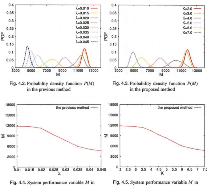
Figures 4.2 and 4.3 show the probability distribution P(M) for different values of parameter A and K in the previous method and the proposed method, respectively. This figures show that it is possible to control the probability distribution P(M) in the proposed method similar to the previous method by adjusting the control parameter K.

Figures 4.4 and 4.5 show the system performance variable M for different values of parameters A and K in the previous method and the proposed method, respectively. In the proposed method, if the control parameter K increase, the system performance variable M takes small value similar to the previous method. According to these figures, efficacy of the proposed method is confirmed.

(26)

4.2 Characteristic of the Proposed Method 21

LL a a

0.4

?.=0.010 - 0.35X=0.015

X=0.020 ...

0.3X =0.025

0.25A=0.030

X=0.035

0.2X=0 .040

0.15X=0.045 - - ••

: L

0.1;•

0.05

8p.:.. 0005000 7000 9000 11000 13000 M

Fig. 4.2. Probability density function P(M) in the previous method

U- 0 a

0.4 0.35

0.3 0.25

0.2 0.15

0.1 0.05

3

K=2.0 K=3.0 K=4.0 K=5.0 K=6.0 K=7.0

3000 5000 7000 9000 11000

M

Fig. 4.3. Probability density function in the proposed method

13000

P(M)

18000

15000

12000

M 9000 6000

3000

%.101 0.015 0.02 0.025 0.03 0.035 0.04

A.

Fig. 4.4. System performance variable M in the previous method

18000

15000

12000

M 9000

0.045 6000

3000

2 2.5 3 3.5 4 4.5 5 5.5 6 6.5 7 7.5 K

Fig. 4.5. System performance variable M in the proposed method

4.2.2 Balance of VM Concentration and Decentralization

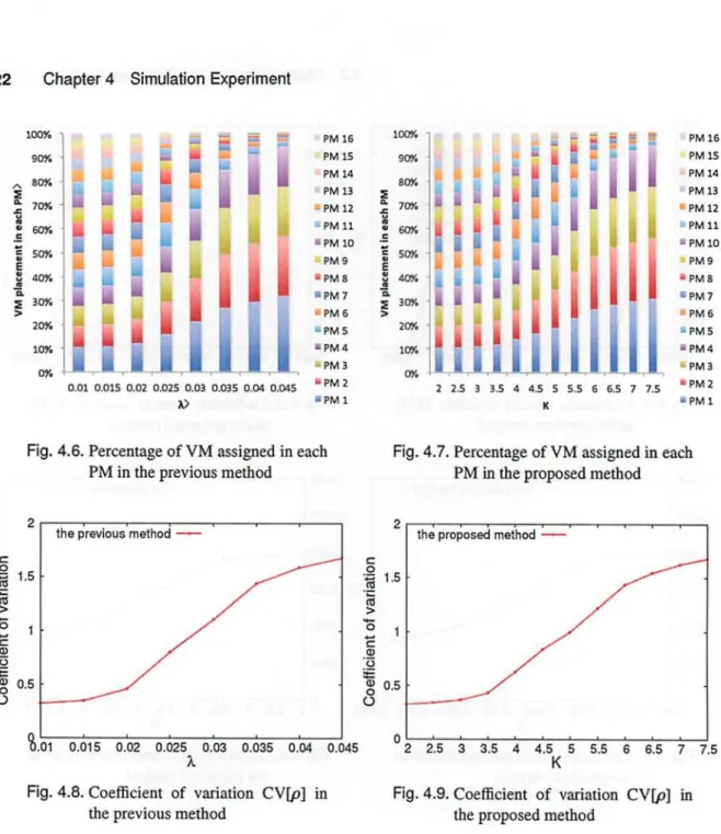
Figures 4.6 and 4.7 show percentage of VM assigned in each PM for different values of parameters A and K when using the previous method and proposed method, respectively. This figures show that the VM concentration becomes strong as both control parameters increase. In addition, figures 4.8 and 4.9 show coefficient of variation CV [p] for different values of control parameters A and K when using the previous method and proposed method, respectively. These figures show that the VM concentration becomes strong as both control parameters increase.

Figure 4.10 shows the system performance variable M for each coefficient of variation CV[p]

when using the previous method and proposed method. This figure shows that large M corresponds to the small CV [p], and small M corresponds to the large CV [p] linearly. In addition, the

(27)

22 Chapter 4 Simulation Experiment

1.

s V

C C 0 E 0

if 0.

2 100%

90%

80%

70%

60%

50%

40%

30%

20%

10%

0%

i

1 ^is

illI II

I

II

0.01 0.015 0.02

C

Y

r.7

0.025 0.03 0.035 0.04 0.045 A>

PM 16 PM 15 PM 14

• PM 13 wPM12 6m11

•m10 -PM9

•PM8

•PM7

•PM6

•PM5

•PM4 .PM3

•PM2

^ PM 1

V F.

O 0 e e Y

E Y a 2

100%

90%

80%

70%

60%

50%

40%

30%

20%

10%

0%

^. ii ! Oh Li 14 111

I M~

I at

ii'

i

r Y

2 2.5 3 3.5 4 4.5 5 5.5 6 6.5 7 7.5 IC

PM 16 PM 15 PM 14

• PM 13 1,PM12

LAPM11

•PM10 PM9

• PM 8

•PM7

•PM6

• PM 5

• PM 4 PM3

•PM2

•PM1

Fig. 4.6. Percentage of VM assigned in each PM in the previous method

Fig. 4.7. Percentage of VM assigned in each PM in the proposed method

2

: t5

O..1

c m 0.5 U

%.01 0.015 0.02 0.025 0.03 0.035 0.04 Fig. 4.8. Coefficient of variation CV[p] in

the previous method

0.045 2

c o 1 . 5 .c

al 15 1 c m 75

00.5

U

0 2 2

.5 3 3.5 4 4.5 5 5.5 6 6.5 7 7.5 K

Fig. 4.9. Coefficient of variation CV[p] in the proposed method

proposed method has the similar characteristic with the previous method, that VMs having high traffic rate are assigned in same or near PM.

According to these figures, it is confirmed that the control parameter K is useful for adjusting the VM concentration.