Biogenic Sources of Sulfur Emission to the Atmosphere and Their On-Site Measurement
Methods
Md. Abul Kalam Azad
Dissertation submitted to the Graduate School of Science and Technology, Kumamoto University in partial fulfillment of the requirements for the degree of
Doctor of Philosophy
September, 2006 Kumamoto, Japan
(Dedicated
My parents
Abstract:
Biogenic Sources of Sulfur Emission to the Atmosphere and Their On-Site Measurement Methods.
Volatile sulfur compounds (VSCs) are emitted to the atmosphere from both natural and anthropogenic sources. Identification and characterization of sources of atmospheric natural sulfur compounds are essential for the rational formulation of emission control policies design to limit the atmospheric sulfate burden, for analysis of the origins of acidic precipitation, and exploring global climate change. It is a challenge for analytical chemist to analyze VSCs at trace levels in the field because of their highly adsorptive, reactive and volatile properties. In the present research, I have investigated some natural sources of hydrogen sulfide, sulfiir dioxide and development of new analytical method for on-site measurement of volatile sulfur gases methyl mercaptan and dimethyl sulfide.
Emission variability of hydrogen sulfide and sulfur dioxide from tidal flat sediments to atmosphere in Ariake Sea, Japan was studied using a diffusion scrubber-based portable instrument. Ariake Sea is a typical closed sea consisting of a huge marsh area along the coast.
Seasonal, spatial and diurnal variability in emission rates were examined. In addition, depth profiles of the gas emissions were examined with the profiles of anions, heavy metals, water and organic contents. Unexpectedly, SO2 emission was much higher than H2S in all measurements, while an opposite emission trend was observed in diurnal and spatial patterns of H2S and SO2 emissions. The mechanisms of these gas emissions are discussed. Total sulfur fluxes to the atmosphere as H2S and SO2 during the study averaged 7.1 jigSm'2 h'1 for muddy sites and 28 jigSm" h" for sandy sites. Estimated total sulfiir turnover in the whole tidal land of Ariake Sea was 20.2 t S y1. Sulfur fluxes from tidal flats were comparable to
the artificial sulfur emission from the neighboring towns.
Emission of hydrogen sulfide and sulfur dioxide from agricultural soils were studied by using model agricultural field and concentration of these gases in the volcanic gases at Mt.
Aso. Emission was investigated from model agricultural field with and without fertilizer.
Emission variability also observed with respect to soil physical characteristics. Mean emission rate as SO2 and H2S from the four different model fields were 23.98 ± 14.17 and 2.07 ± 3.46 (without fertilizer), 29.39 ± 14.25 and 2.09 ± 4.14 (natural fertilizer), 7.81 ± 5.05
and 2.09 ± 3.98 (chemical fertilizer), 9.02 ± 7.83 and 2.63 ± 4.57 |igS m"2 h"1 (mixed iii
fertilizer) obtained. Emission of H2S was stable during the measurement period. Very high fluctuation of SO2 emission was observed compare to the emission of H2S. SO2 emission was significantly influenced by the soil physical properties e.g. soil moisture content and soil surface temperature. Significant emission was observed from this kind of agricultural field, although, the mechanism of emission is not clear. In active period of volcano, concentration of SO2 and H2S were significantly increased. SO2 concentration was increased up to 15 ppmv whereas H2S concentration increased up to 1 ppmv.
Simple and automated method for measurement of methyl mercaptan (CH3SH) and dimethyl sulfide (DMS) has been investigated. These two are the most odorous among the sulfur gases. The collection and subsequently separation are performed with a single short column packed with silica gel adsorbent without any additional separation column. CH3SH and DMS were separated according to their desorption temperatures and introduced into a chemiluminescence cell in the same order. These two gases were detected based on the strong gas phase chemiluminescence reaction with ozone. Linearity of calibration curves with this system is advantageous compared to flame photometric detector. The total system, including a small cylinder for the carrier nitrogen, can be set in a carriable box. The instrument is applicable to breath odor analysis. Also, automated and continuous measurement of room air could be performed with this instrument. During continuous three days toilet air analysis by the reported instrument, it was observed that the sulfur gases level increased after becoming dark. The sulfur gases in ppbv level were successfully measured without any big interference and complicated experimental procedure. Limit of detection of the method for CH3SH and DMS was 0.3 and 0.05 ppb respectively.
IV
Acknowledgements
This dissertation could not have been written without Dr. Kei Toda who not only served as my supervisor but also encouraged and challenged me throughout my academic program. I owe a great deal to my advisor. I would like to extend my deepest thanks and appreciation to my advisor for his ideas and suggestions for solving obstacles encountered during my research. His supervision and encouragement has helped me to fulfill my goal in graduate research.
I would like to acknowledge my gratefulness to Professor Isao Sanemasa for his instructions and encouragements.
I would like to thank the members of my advisory committee, Professor Masayuki Takamiya, Professor Kimiaki Imafuku and Professor Noriyuki Momoshima for their time and guidance through my graduate study at Kumamoto University.
I am indebted to all of the students of Toda group (both current and former) particularly Dr.
Shin-Ichi Ohira for their support, and helpful suggestions during my research work. I really enjoyed their companies.
I would also like to thank Ministry of Education, Sports and Culture, Japan to provide financial support for carrying out this research.
I express my deepest thanks and appreciation to my wife, Nelufa Yesmin, whose moral support was essential for the completion of my studies.
Finally, I would like to express my deepest gratitude to my parents, daughter as well as all of my relatives and well-wishers who have always supported me through all of life's endeavors.
Table of Contents
CHAPTER 1. Introduction to Global Sulfur Cycle.
1.1. Introduction and Overview of Global Sulfur Cycle 1 1.2. Sulfur Gases and Their Role in Global Sulfur Cycle 5 1.3. Impact ofAtmospheric Sulfur to the Local and Global
Environment 5
1.4. Sources of Sulfiir to the Atmosphere 6
1.4.1. Anthropogenic Sources 6
1.4.2. Natural Sources 6
1.4.3. Significance of Natural Sulfur Sources to the Global
Sulfur Cycle 6
1.5. Necessity of Measurement ofNatural Sulfiir Emission 6
1.6. Conclusions 7
References 8
CHAPTER 2. On-Site Measurement of Hydrogen Sulfide and Sulfur Dioxide Emission from Tidal Flat Sediment of Ariake Sea, Japan
2.1. Abstract 10
2.2. Introduction 10
2.3. Materials and Methods 12
2.3.1. Sampling Sites 12
2.3.2. Instrument for On-Site Measurement 14 2.3.3 Instrument Used in the Present Gas Measurement
System 14
2.3.4. Emission Measurement Procedure at Sediment-
Atmosphere Interface 17
2.3.5. Depth Profile Measurement of Soil Gases 18 2.3.6. Determination of Physical and Chemical
Characteristics of Sediments 18
2.4. Results and Discussion • 18
VI
2.4.1. Sediments Characteristics of Ariake Sea 18
2.4.2. Spatial Emission Variation 20
2.4.3. Seasonal Variation of H2S and SO2 Fluxes 20 2.4.4. Diurnal Variation of H2S and SO2 Fluxes 22 2.4.5. Vertical Distribution of Active Ions and Gas
Emission 23
2.4.6. Emission of H2S 24
2.4.7. Emission of SO2 26
2.4.8. Total Sulfur Flux to the Atmosphere 27
2.5. Conclusions 29
References 30
CHAPTER 3. The Measurement of Natural Hydrogen Sulfide and Sulfur Dioxide Emission from Agricultural Soil and Volcanic Gases at Mt. Aso.
3.1. Abstract 32
3.2. Introduction • 32
3.3. Materials and Methods 33
3.3.1. Preparation ofAgriculture Field and Measurement of
Soil Properties 33
3.3.2. Dynamic Chamber Sampling System and Instrument
for On-Site Emission Measurement 34
3.4. Results and Discussion 38
3.4.1. Measurement of Gas Emission 38
3.4.2. Effect of Fertilizer on Emission of Gases 39 3.4.3. Effect of Soil Moisture Content and Atmospheric
Weather Condition on Emission 40
3.4.4. Global Implications to Sulfur Emission 41 3.4.5. Measurement of SO2 and H2S at Mt. Aso 41
3.5. Conclusions 43
References 44
vn
CHAPTER 4. On-Site Measurement of Methyl Mercaptan and Dimethyl Sulfide Single Column Trapping/Separation and Chemiluminescence Detection
4.1. Abstract 45
4.2. Introduction 45
4.3. Experimental 47
4.3.1. Trapping/Separation Column 47
4.3.2. Chemiluminescence Detector 47
4.3.3. Instrumentation and Measurement Procedure 52
4.3.4. Test Gas Preparation 55
4.3.5. Sample Measurements 59
4.3.6. Comparable Measurements With GC-FPD 59
4.4. Results and Discussion 59
4.4.1. Chemiluminescence Reaction Cell 59
4.4.2. Mini-Column for Trap and Separation 60 4.4.3 Performance of The Measurement System 64
4.4.4. Interference from Diverse Gases 66
4.4.5. Application to Breath Odor and Septic Tank
Headspace Gas Analysis 69
4.4.6. Automated Measurements of Toilet Air and Emission
from Tidal Flat Sediment 73
4.5. Conclusions 77
References 78
CHAPTER 5. Research Perspective and Suggestion for Future Work 81
Appendix 82
vni
CHAPTER 1
Introduction to Global Sulfur Cycle
1.1. Introduction and Overview of Global Sulfur Cycle
Sulfur is one of the constituents of many proteins, vitamins and hormones. It recycles like other biogeochemical cycles.
The essential steps ofthe sulfur cycle are:
• Mineralization of organic sulfur to the inorganic form, hydrogen sulfide: (H2S).
• Oxidation of sulfide and elemental sulfur (S) and related compounds to sulfate
(SO42).
• Reduction of sulfate to sulfide.
• Microbial immobilization of the sulfur compounds and subsequent incorporation into the organic form of sulfur.
Overview: Important reactions of the sulfur cycle
S Assimilative sulfate reduction in which sulfate (SO42) is reduced to organic
sulfhydryl groups (R-SH) by plants, fungi and various prokaryotes. The oxidation states of sulfur are +6 in sulfate and -2 in R-SH.
V Desulfuration in which organic molecules containing sulfur can be desulfurated, producing hydrogen sulfide gas (H2S), oxidation state = -2.
Note the similarity to deamination.
S Oxidation of hydrogen sulfide produces elemental sulfur (S°), oxidation state
= 0. This reaction is done by the photosynthetic green and purple sulfur bacteria and some chemolithotrophs.
S Further oxidation ofelemental sulfur by sulfur oxidizers produces sulfate.
S Dissimilative sulfur reduction in which elemental sulfur can be reduced to hydrogen sulfide.
S Dissimilative sulfate reduction in which sulfate reducers generate hydrogen sulfide from sulfate.
Reservoirs of sulfur atoms:
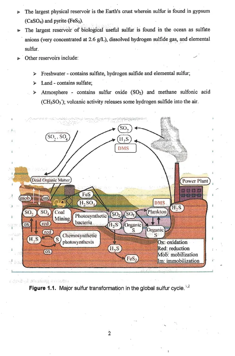
*• The largest physical reservoir is the Earth's crust wherein suliur is found in gypsum (Ca&O^) and pyrite (FeS2>.
.*»■ The largest reservoir of biological useful sulfur is found in the ocean as sulfate anions (very concentrated at 2.6 g/L), dissolved hydrogen sulfide gas, and elemental sulfur.
*■ Other reservoirs include:
> Freshwater - contains sulfate, hydrogen sulfide and elemental sulfur;
> Land - contains sulfate;
> Atmosphere - contains sulfur oxide (S.O2) and methane sulfonic acid (CH3SO3"); volcanic activity releases some hydrogen sulfide into the air.
iP&wer Plant)
^ ■.... ,^ -■-
Chemosynthetic
photosynthesis fjOx: oxidation
|JR.ed: reduction KJMbb: mobilization
«Hm: immobilization
Figure 1.1. Major sulfur transformation in the global sulfur cycle.'2
!o
Given that Sulfur Is "Already Fixed", Why Bother Studying the Sulfur Cycle?
1. Environmental impacts are diverse and important locally even on a human time scale:
a. Some of the reactions that occur in the sulfur cycle open up new environments to life. They support biological communities in unlikely places such as deep sea thermal vents, areas of low pH and areas of high
temperature.
b, On the other hand, certain reactions remove needed metabolites or produce wastes that make environments uninhabitable to some organisms.
2. Interesting microbial chemistries, that no other organisms do, are found in cycles such as the sulfur cycle. They have been exploited in:
a. Mining,
b. Bioremediation,
c. Synthesis of industrial chemicals.
Human impact on the sulfur cycle is primarily in the production of sulfur dioxide (SO2) from industry (e.g. burning coal) and the internal combustion engine. Sulfur dioxide can precipitate onto surfaces where it can be oxidized to sulfate in the soil (it is also toxic to some plants), reduced to sulfide in the atmosphere, or oxidized to sulfate in the atmosphere through photochemical oxidation as sulfuric acid, a principal component of acid rain.
1
ftsiflfltt, dry iJ-apa
i
Sea sail feran
jceans
30, aid lit
■'■■
1.15 V (Rai o SO, sn:i $u|{sf#f
__. ..:V,v ,-. ■'■;;.,:.;■
1 si»ii and. ;
VblttittS
:^|: "■•; Si :■!?■■:
■■i,s. so,
■ ---
:.■■.' '
% Some 8B ftoiE
■; y ■■-
-
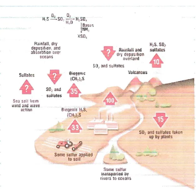
rtteis io
Figure 1.2. Global atmospheric sulfur cycle. Fluxes of sulfur represented by the arrows are in millions metric tons per year. Those marked with a question mark are uncertain, but large, probably of the order of 100 million metric tons per year.
1.2. Sulfur Gases and Their Role in Global Sulfur Cycle
Sulfur-gases in the^afeiosphere iadude hydrogen sulfide {HaS).; carbenyl sulfide (COS), carbon disuMde (CS2), methyl mercaptan (CH3SH), dimethyl sulfide (DMS), sulfur dioxide (SO2) and so on..They plays crucial role to the global sulfur cycle. They are emitted to.the atmosphere from natural and anthropogenic sources through wide variety of complex chemical and biochemical processes and deposited to the earth by wet and dry deposition
system.
1.3. Impact of Atmospheric Sulfur to the Local and Global Environment
It is known that both natural -asd-man-made sources release chemical species that «an modify acidic deposition, climate, human health, ecological systems', and visibility. The study ofthe sulfur cycle has received much attention during recent decades since, apart from its climatic relevance, sulfur via non-sea-salt sulfate is the main contributor to acidity of both wet and dry deposition at urban as well as at remote ofthe world. ■'"J
Agriculture, urbanization and releases of various chemical substances into the soil, air and water have altered our environment on local, regional and global scales. In particular, sulfur emissions have grown rapidly and extensive research has documented a Variety of effects on the environment. Sulfur emissions play a crucial role in three important environmental problems: local air pollution and smog, acid rain and dry deposition, arid global climate change. Not only SO2 but also reduced sulfur compounds can undergo Chemical and photochemical oxidation to yield compound such as methanesulfanic and sulfuric aeid.^
Their increases are important because sulfur gases are oxidized in the atmosphere with the formation of sulfate; resulting in environmental problems associated with the acid rain.
Those sulfur gases may participate and disturb the natural transfer of sulfur of biological origin." It is also evident that sulfur gases play an important role in the forriiatiori and growth of aerosol particles in the troposphere: they may alter the optical properties of clouds
which may interfere with global climate change.9"11 Sulfate aerosol may also provide surfaces for heterogeneous reactions that could affect stratospheric ozone levels." n
The Intergovernmental Panel on Climate Change (JPCG) report (1PCC, 1994) reconfirmed the ability of aerosols to alter climate by changing the radiative balance ofthe atmosphere.
In addition, sulfur-containing odorants are subject to strong public criticism.
Consequently, volatile sulfur compounds are important in the atmospheric environment.
1.4. Sources of Sulfur to the Atmosphere
Sulfur in the atmosphere originates either from natural processes or anthropogenic activity.
■ ■• ' ■■ ' ■■ ■ ■ ■ ■ '
1.4.1. Anthropogenic Sources
Approximately 100 millions metric tones of sulfur per year enters the global atmosphere through anthropogenic activities, primarily as SO2 from the combustion of coal and residual fuel oil.J
1.4.2. Natural Sources
Several author reported that natural sources are constitute a large fraction of the atmospheric sulfur burdea14"10 The major sources of natural sulfur emission are coastal and wetland, ecosystems, vegetation, plant and inland soil, oceanic environments, volcanic
activity, biomassburning.17-20 ,f .
1.4.3. Significance of Natural Sulfur Sources to the Global Sulfur Cycle
In biogeochemistryj the sulfur cycle is one of the most complex cycles because oxidation of sulfur varies between - 2 and + 6 and there are a large variety of organic and inorganic species. Large uncertainties remain concerning the chemical species and the magnitude of natural emission of sulfur gases into the atmosphere: Biogenie sulfur that is sulfur compounds which result from biological processes are a vital sources of sulfur to the atmosphere. The annual amounts of sulfur evolved .from biogenic sources have been
estimated to be 15t50 Tg S yr"1.2' Bates eiai reportedthat contribution ofnatural sources to the global sulfur emission is estimates as 62%." Identification and characterization of sources of atmospheric natural sulfur compounds are essential for the rational formulation of emission control policies design to limit the atmospheric sulfate burden, for analysis of the origins of acidic precipitation, and exploring global climate change. The significance of the anthropogenic sulfur emissions as well as the climatic importance in the natural sulfur cycle is difficult to assess without first quantifying the sulfur emission from natural sources. Due to this reason, there is a special significance for the investigation on the natural emission of sulfur gases.
1.5. Necessity of Measurement of Natural Sulfur Emission:
Sulfur species emitted from both natural and man-made sources can modify acidic deposition, climate, human health etc. If a controlled reduction in mane-made emissions
6
were to occur, natural sources would continue to affect acidic deposition, climate, human health and welfare. As a result, the benefits that would be anticipated from such a controlled reduction could be erroneously optimistic if natural sources make a significant contribution to the present total acidic, climatic and atmospheric budget. Therefore, policy decisions regarding possible emission control strategies require, among other inputs, an accurate assessment ofthe relative importance of natural and man-made sources.
Data on sulfur emissions are important for analyzing and understanding three important environmental problems: local air pollution and smog, acid rain and dry deposition, and
global climate change. ■■...-'
In all the early attempts at developing global sulfur budgets, natural emissions were obtained from the amount of sulfur necessary to balance the cycle.. This* resulted in
considerable scatter in the biogenic estimates, from 34 to 267 fg S yr"1.22 It is possible with
the existing data to begin to make estimates of the upper and lower bounds for biogenic
emissions based on direct measurements 30 However, additional data are necessary to asses
biogenic sulfur emissions independent ofthe other portions ofthe global sulfur cycle.
■■'..- : ■■ ■ ■".■■■ ,-■.■■■ ■■ ■ -■,'-.
1.6. Conclusions
;;.To improve the estimation of global natural sulfur emission to the atmosphere, accurate measurement of natural sulfur flux is required. Attempts to estimate natural sulfur emissions have been fraught with both a paucity of data and high natural Variability. Moreover, the emissions from plants and inland soils, may play a significant role in global sulfur cycling and very little work has been reported covering this subject, In the present research emission of sulfur gases from natural sources and their on-site measurement method has been investigated.
References
1. Smith, R., Smith, T., Elements ofEcology, Scientific Publishing Services Limited, UK pp.200.
2. Andreae, M.O., Crutzer, PJ., Atmospheric aerosol: biogeochemical sources and role in atmospheric chemistry. Science, 276, pp. 1052-1058 (1997)
3. Smith, R.L.; Smith, T.M.; Hickman, G.C.; Hickman, S.M.; Manahan, E.S., Environmental Chemistry, (Seventh Edition), Lewis Publisher, New York, pp.331 (2000).
4. Stanier, R.Y., Doudoroff, M, Adelberg, E.A., 1970. The microbial world, pp.698-699.
Prentice-Hall, Inc., Englewood cliffs, New Jersey.
5. Charlson, R. J. and Rodhe, H. Factors controlling the acidity of natural rainwater.
Nature, 295, pp.683-685 (1982).
6. Galloway, J. N., Likens, G. E., Keene, W. C. and Miller,J.M. The composition of precipitation in remote areas of the world. Journal of Geophysical Research, 87, pp.8771-8786 (1982).
7. Rodhe, H. Human impact on the atmospheric sulfur balance. Tellus, 51A-B, pp. 110—
122 (1999).
8. Kiene, R. P., Production of methanethiol from dimethylsulfoniopropionate in marine surface waters. Marine Chemistry, 54 (1-2), pp.69-83 (1996).
9. Charlson R. I, Lovelock J. E., Andreae M. O. and Warren S. G. Oceanic phytoplankton, atmospheric sulfur, cloud albedo and climate. Nature, 326, pp.655-661 (1987).
10. Aneja V. P., Natural sulfur emissions into the atmosphere. Journal of Air and Waste Management Association, 40, pp.469-476 (1990).
11. Minami K., Kanda K. and Tsuruta H. Emission of biogenic sulfur gases from rice paddies in Japan. In The Biogeochemistry of Global Change (edited by Oremland R. S.), pp.405-418. Chapman & Hall, New York. (1993).
12. Lovelock J. E., Maggs R. J. and Rasmussen R. A. Atmospheric DMS and their natural sulflir cycle. Nature, 231, pp.452 -453 (1972).
13. Charlson R. J., Langner J. and Rodhe H. Sulfur aerosol and climate. Nature, 348, pp.22 (1990).
14. Chin, M, Davis, D.D. A reanalysis of carbonyl sulfide as a source of stratospheric background sulfur aerosol. Journal of Geophysical Research, 100, pp.8993-9005 (1995).
15. Goss, L.M., Frost, G.J., Donaldson, D.J., Vaida, V. Photooxidation of CS2 in the near- ultraviolet and its atmospheric implications. Geophysical Research Letters, 22, pp.2609-2612 (1995).
16. Bodenbender J., Wassmann R., Papen H., Rennenberg H. Temporal and spatial variation of sulfur-gas-transfer between coastal marine sediments and the atmosphere.
Atmospheric Environment, 33, pp.3487-3502 (1999).
17. Goldan, P.D.; Kuster, W.C.; Albritton, D.L.; Fehsenfeld, F.C. The measurement of Natural sulfur emissions from soils and vegetation: Three sites in the eastern United
States revised. Journal ofAtmospheric Chemistry, 5, pp.439-467 (1987).
18. Bates, T,B.; Lamb,B.K.; Guenther,A.; Dignon, J.; Stoiber, R.E., Sulfiir Emissions to the Atmosphere from Natural Sources, Journal ofAtmospheric Chemistry, 14, pp.315- 337 (1992).
19. Macdonald, B. T. C, Denmed, O. T., White, I., Melville, M. D. Natural sulfur dioxide emissions from sulfuric soils. Atmospheric Environment, 38, pp. 1473-1480 (2004).
20. Watson, R.T., Meira Filho, L.G., Sanhueza, E., Janetos, A., 1992. Climate Change 1992:
The Supplementary Report to the IPCC Scientific Assessment. Cambridge University
Press, Cambridge, pp. 25^6. ;
8
21. Simo, R., Production of atmospheric sulfur by oceanic plankton: biogeochemical, ecological and evolutionary links. TRENDS in Ecology & Evolution, 16 (6), pp.287-294 (2001).
22. Eriksson, E., The yearly circulation of chloride and sulfur in nature; metrological, geochemical and pedological implications. Tellus, 12, pp.63 (1960)
CHAPTER 2
On-Site Measurement of Hydrogen Suffide and Sulfur Dioxide Emission from Tidal Flat Sediment of Ariake Sea, Japan
2.1. Abstract
Emission variability of hydrogen sulfide and sulfur dioxide from tidal flat sediments to atmosphere in Ariake Sea, Japan was studied using a diffusion scrubber-based portable instrument. Ariake Sea is a typical closed sea consisting of a huge marsh area along the coast. Seasonal, spatial and diurnal variability in emission rates were examined. In addition, depth profiles of the gas emissions were examined with the profiles of anions, heavy metals, water and organic contents. Unexpectedly, SO2 emission was much higher than H2S in all measurements, while an opposite emission trend was observed in diurnal and spatial patterns of H2S and SO2 emissions. The mechanisms of these gas emissions are discussed. Total
O 1
sulfur fluxes to the atmosphere as H2S and SO2 during the study averaged 7.1 ugS m~ h"
for muddy sites and 28 \igS m"2 h"r for sandy sites. Sulfur fluxes from tidal flats were
comparable to the artificial sulfur emission from the neighboring towns.
2.2. Introduction
Ariake Sea is one of the best-known semi-closed seas in Japan and has unique features.
Its tidal area is the largest in Japan. Tidal range at the flood tide is about 3 m in the bay mouth area, and it becomes bigger in the bay head area with the tidal range of 4.5-5 m.
Many rivers flow into the eastern coast area of Ariake Sea and carry 440,000 tons of sediments per year. Big grain sediments accumulate in the eastern coast, and minute grains are- brought by the-residual- carrent and accumulate-in-the-bay head to- form vast tidal flats with fine sediments.1 Rivers load nutrients and organic waste into the tidal flats. On the
other hand, seawater supplies sulfate periodically. In these situations, sulfur gases are supposed to emit largely from coastal sediments. However, there has been no quantitative study on- bipgenk- sttMuf emtsskMar from- tidal- flats of Ariake- Sea: Environmental issues
related to Ariake Sea have been a topic of increasing interest recently1"3 and analysis of
characteristics of tidal flats is of great interest to the regional population.
Reducing sulfur gases, such as hydrogen sulfide (H2S), methylmercaptan (CH3SH) and dimethylsulfide (DMS) and so on, involves chemical and" photochemical oxidations to yield methanesulfonate and sulfuric acibV-4t is recognized that not only sulfur dioxide (SO2), but
10
also these reducing sulfur gases contribute largely to the formation and growth of aerosol particles in the troposphere. These aerosols are thought to alter the optical properties and contribute to acid deposition and cloud formation, which may interfere with the global climate change. ' The increasing interest in studying natural sulfur emission has become important over the last two decades because of its significant role in the global sulfur cycles.
Estimations of natural sulfur emissions were reported to be equivalent to anthropogenic
emissions,910 drawing the attention to the contribution of biogenic sources of volatile reduced sulfur compounds to the global sulfur cycles. Several attempts have been made to measure biogenic sulfur gas emissions from European and American soils and coastal
marshes. l1"J/ H2S andDMS are the dominant gases emitted from coastal marshes.15 DMS is
the dominant gas released from grass and. algae, whereas mostly H2S is emitted from
intertidal mud flats.19 On the other hand, direct emission of SO2 from marsh sediments has not been discussed in detail. In a recent report, MscdonnM et'al*} showed that soils have long been recognized as the sink of SO2 while soils could be a source. They reported SO2 emission from acid sulfate soils in Australia as an initial field measurement. An interesting issue that is worth investigating is whether SO2 is emitted or not, directly from normal neutral soils. In the present work, emission of SO2 was measured together with H2S, the dominant reduced sulfur gas, in tidal flats of Ariake Sea, Japan. Both H2S and SO2 were simultaneously measured on site at the tideland using a portable instrument that was modified for this purpose. Measurement of sulfur gases is generally complicated with
analytical methodological difficulties.10 In most measurements of sulfur gas emission; the sample is collected, preconcentrated into a column, and then purged to be measured by gas chromatography. In this study, the gases were measured directly on site. The method used was easy to conduct and suitable for field measurement. ,
11
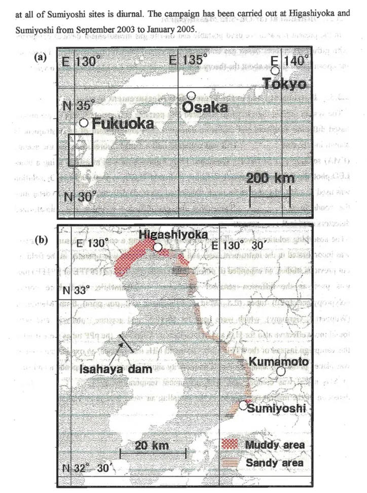
at all of Sumiyoshi sites is diurnal. The campaign has been carried out at Higashiyoka and
>' ' ' ■ ■ . '
Sumiyoshi from September 2003 to January 2005.,
(a)
fl
■:->
'■
■ ■■ .■ ■."■■
.:■•,,-- '. ;
(b)
■
■
N
fflt
■.--■.■■■■.;: ■:■-.:;;• i. <;■■■..-
N
E 130* asiiiyoka
33'
■-■ :i'
m
Isahaya dam
'VI :
32" 30'
1
130° 30'
... ■: , ■:':■■■, .v : l .:. ■-■ i 'v: ?■■■.••■•■■ i
' , ■ ■ s
diT
M Sandy area
: ■
■■-■ .- . •
:;■ -■ ■■ '..:
i ■■■
: • - .
. '■ .. ." ■
: ■ ■
- .
•■■ ■ .
i
Figure 2.2. Location of Ariake Sea in Kyushu island, Japan (a), sampling sites along the coast of Ariake Sea in the muddy and sandy tidal flat area (b).
13
2.3.2. Instrument for On-Site Measurement
In the present research we used portable and on-site gas measurement devices comprised with diffusion scrubber based gas collection system and miniaturized detectors. Please see the appendix for details about the theory of diffusion scrubber based gas collection system.
■
2.3.3. Instrument Used in the Present Gas Measurement System
The system used in the campaign consisted of a portable device comprising of membrane
based diffusion scrubbers and miniature detectors.21"23 Flow diagram of the instrument is
shown in a box of Figure 2.3. FfeS was collected into a 1 mM fluorescein mercuric acetate (FMA) solution (0.1 M NaOH). Quenched FMA fluorescence was measured using a blue- LED/photodiode-based homemade detector. A 5 mM H2SO4 with 0.006% H2O2 solution was used as a SQ2 absorber and a micro-fabricated electrode detector was used to determine the conductivity. Figure 2.6 Shows that the gas diffusion scrubber and miniaturized
detectors used in the instrument. %
The absorbing solutions were allowed to flow by applying a constant pressure. A battery was incorporated in the instrument case, and the whole system was operated in the field. In
our previous studies,- an expanded or porous polytetrafluoroethylene (ePTFJ^or pPTFE) tube was used as the diffusion scrubber membrane.22>23 Meanwhile, small bore porous polypropylene (pPP) tubes (0.5 mmid x 0.9 mmod, 0.2 |jm pore) from Membrana (Wuppertal, Germany), which were used for HCHO24 and acetone23 analysis, and were found more effective also for EfeS and SO2 collection. Therefore, the pPP tubes were used in this campaign instead of the PTFE tubes. To avoid NH3 interference, an oxalic acid column was placed in the SO2 sampling line. Conductivity signal is temperature dependent and span
of SO2 signal was compensated with instrument temperature by 1.5% °C'\ Limits of
detection of the instrument in ppbv in the sampling air were 0.02 ppbv H2S and 0.4 ppbv SO2.
14
:
Chamber
A(r| 1 HP?
IIP
Sediment
12 V
Battery •
data logger
Control circuit board
RB1 RB2 B
instrument Jiox
WB
Fffl
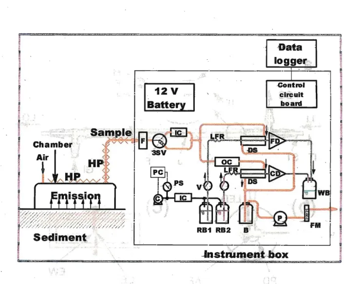
Figure 2.3. Schematic diagram of the sampling/measurement system for simultaneous measurements of H2S and SO2 emissions at tidal flats. HP: heating pads, F: inlet filter, 3SV: three-way solenoid valve, IC: iodinated activated charcoal/sodalime column, OC:
oxalic acid column, FM: flow meter, B: flow buffer bottle, P: air pump, PC: pressure control circuit, PS: pressure sensor, C: miniature compressor, RB1: FMA reagent bottle, RB2:
H2SO4/H2O2 reagent bottle, V: stop valve, LFR: liquid flow restiictor, FD: fluorescence detector, CD conductivity detector, WB: waste bottle, "DS: diffusion scrubber wlfli porous polypropylene tube.
■ - :
'
■ ■ -
■
■ ■ ■ ■ . . .
1
. ■ ■
I
■ -. .■ -
■
. ■ ■
15
IT OT '- \ \
IT ST M J F
■■■■ •■■ . ■ GL
..-■■ '■
LJ
t
LED
ii/v ^
(c)
B
Ht^"~
CE EW
■ ■
LI X ALO
- ■
■
■. ■
GL
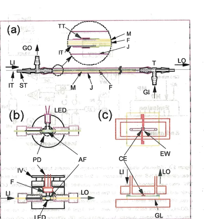
Figure 2.4. Schematic diagram of gas diffusion scrubber and detectors. Parts (a) is structures of scrubber: M, gas permeable membrane tube; J, jacket tube; F, monofilament;
T, tee; IT, inserting tube; ST, spacing tube; TT, Teflon tape; LI, liquid inlet; LO, liquid outlet;
Gl, gas inlet GO, gas outlet. Parts ft)) and (c) are fluorescence detector and conductivity detector, respectively: PD, photodiode; LED, blue LED; F, plastic color filter; AF, Teflon AF tube ceR; fV,
current-to-voltage converting circuit board; CE, conductivity electrode; EW, electrode window; GL, gasket for liquid flow.
16
2.3.4. Emission Measurement Procedure at Sediment-Atmosphere Interface The instrument mentioned above was used for measurement ofthe gases emitted from the sediment surface. A plastic chamber made of polypropylene was used for sampling as shown in the left of Figure 2.3. The chamber was 21 cm w x 28 cm d x 9.5 cm h (sampling
surface area 0.0588 m2, volume of the chamber 5.8 1), and had two ports for air inlet and
outlet. The chamber was placed on the sediment, and air was aspirated from the air outlet to the instrument via a lm Teflon tube (3mmid x 6mmod) at a constant flow rate (2.2-2.5 1
min"1), In order to prevent water condensation, the tube and the upper part of the chamber were kept warm at approximately 50 °C by using heating pads and wrapping them with a plastic sheet. Heating pads are packed with ferric powder and commonly available for healing at drug stores. Usually, a measurement was conducted for 10 min. and ambient levels of H2S and SO2 were 0.2-1.0 ppbv and a few ppbv, respectively, in the campaign field. In the surface measurements, they increased to reach a constant level: H2S level was usually within 2 ppbv (sometimes near 20 ppbv), and SO2 was several to 20 ppbv in the
sampling air. Emission rates, E, in ugS m'2 h"1 were determined from these increases in the gas concentrations (DC, ppbv), the sediment area in the chamber (A, m2) and the total air sampling rate (F, 1 min"1 as the standardized flow at 0 °C and 1 atm):
E= 32.1 xlO^ACxlO"9) (60F)/22.4A r... (2.19)
Usually, the chamber place was changed in the every measurement to avoid increase in temperature by greenhouse effect ofthe chamber. Temperatures ofthe sediments, sample air and the instrument inside were monitored simultaneously with platinum temperature sensors. Calibration of the instrument was performed daily before and after the sampling campaign. Zero-signal was checked at least once in 2 h by passing air through a column packed with iodinated activated charcoal/sodalime. The surface measurements were conducted for investigation of spatial variation in the different sediments in Sumiypshi, seasonal variation at muddy Higashoyoka and sandy Sumiyoshi. Daily variation was examined at typical silty mud sediment in Higashiyoka one time because the repetition of on site measurement overnight was not feasible due to the sampling site being far away from the laboratory and for safety reasons.
17
2.3.5. Depth Profile Measurement of Soil Gases
Depth profile measurements were performed for the sediment at horizontally 18m from the
■■■■■.. ■ . .. ■'
bank in the muddy tidal flat, EBgashiyoka. Sediments (16 kg each) vertically below the surface at 0-2, 10-15, 20-25, 40-45, 60-65, and 80-85 cm depths were sampled into a plastic container (30 cm w x 26 cm d x 16 cm h) and brought back to the bank. The same chamber as the surface measurement was covered onto the sampled sediments, but a sodalime/charcoal column (10mm id x 12 cm L) was placed at the air inlet ofthe chamber to eliminate gases contained in the outside air. Sulfur gases were strongly emitted by vacuum pressure at 87±7 mm H^O generated by aspirating air through the column. After emission peaks appeared then the emission gas levels decreased gradually. Amounts of H2S and SO2
emitted in 10 min aspirating were measured, and emission in ugS kg'1 was obtained from the peak area in the gas concentration vs. time chart, total sampled gas volume and sampled soil weight.
2.3.6. Determination of Physical and Chemical Characteristics of Sediments At the time of the soil sampling for the gas measurement, fresh sediments were taken into airtight polyethylene bags to examine depth profiles of water and organic contents, distribution of sulfide, sulfate and other anions. Water content and bulk organic matter were determined from decrease in weight after drying at 105 °C for 24 h, and loss-on-ignition of dried samples after 6 h at 520 °C.2° For anion analysis, 10 g wet sediments were homogenized with purified water in a test tube, centrifuged and filtered by used a membrane filter. The filtrate was diluted to be 50 ml, and this was used as a sample solution. 5ml ofthe sample solution was mixed with 5ml of20 mM FMA alkaline solution in a test tube, and the fluorescence intensity was measured with a spectrofluorometer (FP-6200, JASCO, Tokyo).
Soluble sulfide was determined from the quenching intensity of FMA fluorescence. Other anions were determined by injection of the sample solution into an ion chromatograph IC (761 Compact IC, Metrhom, Herisau, Swiss) with an anion separation column (Shodex IC
SI-90 4E, 4 mm id x 250 mm long). In case of SCV' and Cl" analyze by IC, the sample was
diluted 200 times prior to the injection.
2.4. Results and Discussions
2.4.1. Sediments Characteristics of Ariake Sea
Higashiyoka is a typical huge muddy site located in the bay head area with sediment particle size ranged from 5 to 50 mm Muddy sediments were neutral (pH 7.4) and showed
18
high water and organic matter contents (62.7 and 4.06%, respectively). We could find a patchy coverage of halophytic plant (Suaeda japonica mikino) only by the bank/7 with an abundance of mudskippers (Boleophthalmus pectinirostris) and lugworms (Neanthea japonica) along the seashore. The other site, Sumiyoshi, was located in the east coast area near the bay mouth, and the sediment type was mainly medium sand but there were partially muddy sand and silt mud. The muddy sand was a transition area, with a 2-5 cm thick coverage of mud and sand mixture and particle size increased with the depth. The muddy sand sediment was observed with abundance of Scopimera globosa and bivalves (Ruditapes philippiriarum).
Table 2.1.
Sediment characteristics of Higashiyoka and Sumiyoshi and mean flux of H2S and S02 to atmosphere from three types of sediment at Sumiyoshi
Particle size (u,m) pH
Water (%) Organic (%) General
Gas emission (p
n
H2S
SO2
Total
Higashiyoka Mud
5-50
■ ■ '; ■ ■ ■■■ ■■''-'.
7.4 62.7 4.06
Patchy coverage of halophytic plants along the bank
LgS m"2 h"1)
Sumiyoshi Mud 5-50
8.4-8.9 60.7
4.16
10
8.97 ±5.5 3
4.98 ±1.30
14.0 ± 5.4
Sandy mud 20-200
7.4-7.6 49.5
2.26 No plant
7
5.49 ±4.5 9
43.0 ± 7.7
48.5 ± 7.5
Sand 100-400
7.4- 7.6 25.1
1.64
10
2.43 ± 0.67
46.1 ±10.
m1
48.5 ± 10.
6
The medium sand sediment was highly water penneable and had low organic matter content as shown in Table 2.1. According to the microscope observation, grain sizes of mud, muddy sand and sand were 5-50, 20-200 and 100-400 mm, respectively. The soil pH of muddy sand and sandy sediments was 7.4-7.6, and muddy sediment pH was 8.4-8.9 at Sumiyoshi.
19
2.4.2. Spatial Emission Variation
Measurements were performed in April to June 2004 at muddy, sandy muddy and sandy sediments all in Sumiyoshi. Distinct emission variability was observed with respect to spatial change as shown in Table 2.1. The highest mean emission rate of H2S was at the
muddy site (8.97±5.53 ugS m^h'1), and the lowest was at the sandy site (2.43±0.61 pigS m'2 h"1); whereas the highest emission rate of SO2 was at the sandy site (46. l±10.7 (igS m"2 h'1), and the lowest was at the muddy site (4.98±1.30 ugS m"2 h"1). Emission of SO2 was
dominant over H2S at the sandy and muddy sites during the measurement period. Kgher fluxes of SO2 were found at the site, which sediments were larger in particle size with low- organic matter content, but higher EfeS fluxes were observed on the sediments of smaller particle size containing high-organic matter.
■ ... r\h ■■-■■■: ;. ■ : •. ;i :■■-■ ■-■■'-_ - -■■"' -: .'■■■' ■' ■■ ■ '■■' ' ■■
: n - .■.,'■■".
2.4.3. Seasonal Variation of H2S and SO2 Fluxes
Emission rates varied with seasonal changes as shown in figure 2,3 (Note that H2S bars are
■■..■■■ ...;■.■-■ ;. - ■ ■_■■.■■
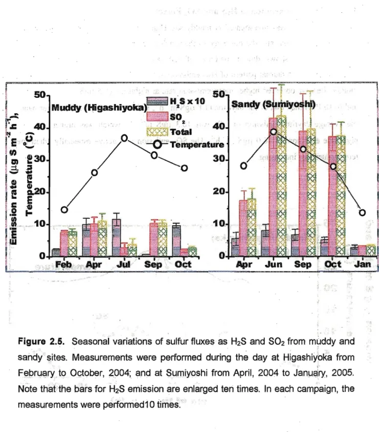
enlarged ten times). They were measured in daytime at muddy site Higashiyoka and sandy site Sumiyoshi. At muddy site, the highest H2S emission was observed in July (1.1670.19
ugS m'2 h"1), and the lowest was in September (0.07±0.01 ugS m"2 h'1). Fluxes of H2S at
muddy site were higher in warmer months, except September, than those in cooler months.
At the same site, the highest SO2 emission was measured in September (10.3±1.0 ugS m"2h'
\ and the lowest in October (1.74±0.53 ugS m"2 h"1). Emission of SO2 did not show any
regular trend with seasonal changes at the muddy site. On the other hand, in the sandy site,
the highest H2S flux was; observed in June (0,81±0.53 ugS m^h'1) and lowest in January (0.29±0.07 |igS m^h'1). Emission rate of SO2 at sandy sites ranged from 3.16±0.11 |j.gS m'2 h"1 (January) to 42.9±9.4 jj.gS m"2 hTl (June). Apparent emission patterns were observed for
both H2S and SO2 at sandy sites with seasonal changes. Emission rates of SO2 were drastically low in winter. The highest emission was observed when the temperature was highest among the measurement campaigns at this site.
20
■
... ■.
50n 50
Muddy (Higashiyoka)
, . T
■ ■ ! - ; • •—
Sandy (S^iijniyo£ hj)
Feb Apr Jul Sep Oct Apr Jun Sep Oct Jan
■ ■■ ■ -
Figure 2.5. Seasonal variations of sulfur fluxes as H2S and SO2 from muddy and sandy sites. Measurements were performed during the day at Higashiyoka from February to October, 2004; and at Sumiyoshi from April, 2004 to January, 2005.
Note that the bars for H2S emission are enlarged ten times. In each campaign, the measurements were performediO times.
21
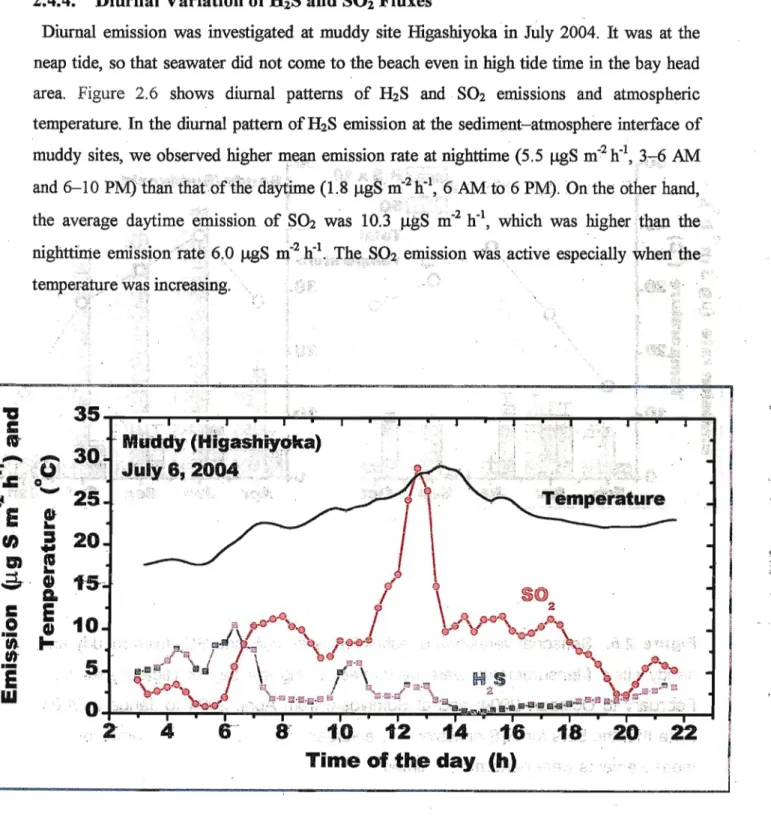
2.4.4. Diurnal Variation of H2S and SO2 Fluxes
Diurnal emission was investigated at muddy site Higashiyoka in July 2004. It was at the neap tide, so that seawater did not come to the beach even in high tide time in the bay head area. Figure 2.6 shows diurnal patterns of H2S and SO2 emissions and atmospheric temperature. In the diurnal pattern of H2S emission at the sediment-atmosphere interface of
muddy sites, we observed higher mean emission rate at nighttime (5.5 ugS m^h"1, 3-6 AM and 6-10 PM) than that of the daytime (1.8 ugS m^h"1, 6 AM to 6 PM). On the other hand, the average daytime emission of SO2 was 10.3 ugS m"2 h"1, which was higher than the nighttime emission rate 6,0 ugS m"2 h"1. The SO2 emission was active especially when the
temperature was increasing.
.
i, ■
■
■ .
1 35
_~ ffi 30
8)
25-
Hi
Muddy (Higashiyoka)
July 6, 2004 - : ■•
■ I |
■■-,
Temperature
- ■■■.:■;
,"3
10 12 14 16 18 20 22 Time of the day (h)
Figure 2.6. Diurnal variations of sulfiir flux. Measurement was performed during the neap tide period at muddy site, Higashiyoka in July, 2004.
22
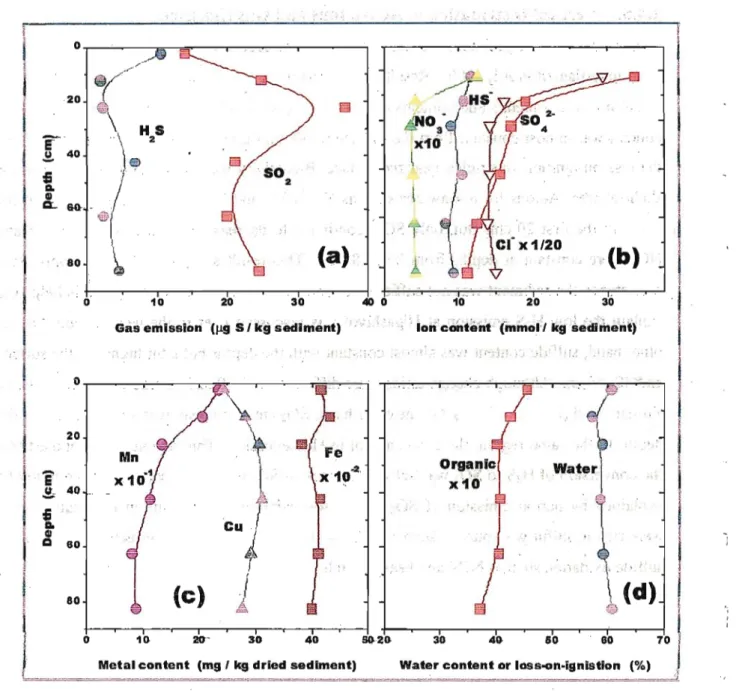
2.4.5. Vertical Distribution of Active Ions and Gas Emission
Gas contents in the sediments vertically below the surface at the silty mud site (Higashiyoka) were investigated in July, 2004. Results are shown in-Figure 2.7 with the vertical distribution of anions, heavy metals and contents of water and organic matter. In these sediments, water content was almost constant from the surface to 80 cm depth. Organic matter obtained from the loss-on-ignition was richer near the surface. Bioactivity was supposed to be higher in the shallow area. Anions from seawater such as Cl", SO42" and NO3" decreased largely with the depth in the first 20 cm. But, only SO42" continued to decrease in deeper area while Cl' and NO3"were constant at depths from 20 to 80 cm This result showed that SO42" supply from seawater to the sediment was not sufficient to generate sulfur gases highly, and this helped to explain the low H2S emission at Higashiyoka as discussed later in the next section. On the other hand, sulfide content was almost constant with the depths but a bit higher in the surface and 40-45 cm: Although change ratios were different but H2S and sulfide contents showed a similar trend (Figure 2.7 a, b). On the other hand, SO2 emission peak was around 20 cm in the depth. In the same region, there was a dent in H2S emission. This region was supposed that the conversion of H2S to SO2 was active. The lack in SO2 emission near the surface might be explained by partial emission of SO2 before soil sampling. Sediments in the shallow area were rich in sulfur gas sources, such as SO42" and organic matters, and effective materials for sulfide oxidation such as NO3' and heavy metals.
■
1
23
£a
Bo 20.
40.
80-
;,
HS 0
0 10 20 30
Gas emission (fig S/ kg sediment)
/iNO3"<
x10
. [
. ■ f * A
'sHS"t~
■ \
1
■ ■
4 t-rJ
r
. -
*»:
X1/20
i * • ■. --'■■
■'■■■■.
(b).:
40 0 10 20 30
Ion content (mmolV kg sediment)
I
20.
40.
60.
60-
x10
Organic
xio Water
tw.
10 29~ 30 40 5a2tt 30 40- 50 60 70
Metal content (mg / kg dried sediment) Water content or loss-on-ignistlon (%) !
Figure 2.7. Depth profile of (a) gas emissions, (b) ions, (c) metals and (d ) organic/water contents. Gas measurement and soil sampling were performed in July 2004 at muddy site, Higashiyoka.
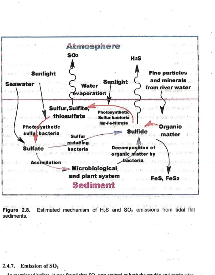
2.4.6. Emission of H2S
Numerous biological and physical parameters govern sulfur cycling in the coastal wetland.
The major sources of reduced sulfur in tidal flat sediments are microbiological sulfate reduction and organic matter decomposition as shown in Figure 2.S Sulfate is supplied to the sediment from seawater. H2S is generated in the sediments from sulfate through activity of the-sulfate1 reducing bacteria. These obligatory anaerobic bacteria oxidize organic compounds and molecular hydrogen by using sulfate as an oxidizing agent."3 In this way, the emission of
24
EfeS is related to the microbial activity. Hence, higher emission rate was observed at muddy sediments in the warmer seasons.
Seasonal emission patterns obtained at Ariake Sea tideland were similar to the data obtained
in Wadden Sea l0 and the estuary ofRiver Come, UK.29 Summer H2S emission rates reported are 66.88±1.72 u,gS m'2 h"1 at Wadden Sea, 13.2 ngS m"2h"J at saltpan of River Colne and 2.33±0.81 ugS m"2 h"1 J7 at Louisiana salt marsh. Our result obtained at Ariake Sea, which was 1.16±0.19 jigS m" h in July at matter was unavailable in our study site. Surface layer of sediments contained 4.56% organic matter (Figure 2.9d). However, the supply of organic matter from seawater to sediment was not achieved everyday, and the remaining organics were supposed to be relatively stable matters. In this way, unavailability of reactive organic matter in the sulfate^reducing zone might also explain the low emission rate.
Oxidation of H2S might be another reason of low emission rate. Kristensen et al 26 found
that close coupling between H2S production near the surface and oxidation by oxygen was the cause of low H2S emission fraction. Most commonly, H2S is removed by chemical oxidation in the underlying sub-oxic zone (or N03"-Mn-Fe zone), and precipitation reactions, which lead to precipitation as FeS and FeS2.30 The high concentration of Mn and NO3" near the sediment surface (Figure 2.7c) substantiates the removal of sulfide through oxidation.
In the diurnal emission pattern (Figure 2.6), oxidation of-sulfide in the^surface sediments might explain the lower H2S emission in daytime compared to that in nighttime. The diurnal emission pattern was similar to data reported by Bodenbender et al for muddy sediments.
They stated that high H2S emission rate during nighttime indicated a shift in the balance between production and consumption processes. The lack of benthic photosynthesis at night suggested that a reduced 02-barrier facilitated H2S transfer from sediments to atmosphere.
Sulfide oxidation (ultimately to sulfate) generally accounts for 50 to 100% of the oxygen consumption in marine sediments.l93) In the case where an O2-H2S interface exists, sulfide oxidation may proceed rapidly and directly via oxygen notably by colorless sulfur bacteria of
the Beggiatoa type.32 Reoxidation of H2S contributes to KfeS removal more than precipitation
as pyrites in marine sediments.lO Interestingly, it is said that 1640-30600 times more H2S are produced than emitted.2"
25
SO2 H2S
Sunlight
Seawater Water
Evaporation
tight
.
Fine particles and minerals from river water
V Phofo^ynthetic
Sulfur,Sulfite,
thiosulfate Photosyntheti Sulfur bacteria
Mn-Fe-Nitrate
■ >
x suif bacteria
Sulfur Sulfide
1
Organic matter
■ n Sulfate
mmreing
bacteria Assimilation
Decomposition of organic matter by
^tfacteriai SVficrobioIogica!
and plant system FeSj FeS?
Figure 2.8. Estimated mechanism of H2S and S02 emissions from tidal flat sediments.
2.4.7. Emission of SO2
As mentioned before, it was found that SO2 was emitted at both the muddy and sandy sites.
Total sul&r emitted from Ariake Sea tidal flat a& SO2 was. 19.6 15.51 S y'1. Interestingly, SO2
was highly emitted even at neutral sediments. Furthermore, SO2 was dominant over H2S at both the muddy and sandy sites during the measurement period. So far, in all investigations on biogenic sulfur gas emission from neutral soil, SO2 data was not presented. Harrison et al.
26