Shock Wave and Condensed Matter Research Center, Kumamoto University, 2-39-1 Kurokami, Kumamoto, 860-8555, JAPAN

Shock analysis of underwater explosion using particle method

Satoshi Matsumoto , Yuichi Nakamura , and Shigeru Itoh

Shock Wave and Condensed Matter Research Center, Kumamoto University, 2-39-1 Kurokami, Kumamoto, 860-8555, JAPAN

corresponding author: [email protected]

Yatsushiro National College of Technology, 2627 Hirayama-shinmachi, Yatsushiro, Kumamoto, 866-8501 JAPAN e-mail: [email protected]

Received: May 27, 2005 Accepted: October 24, 2005

Abstract

A detonation of explosives generates extreme high energy in a very short time. The control of the explosive energy is important to the practical use of explosives. It is one of the most popular techniques to use the underwater shock waves in water. Numerical simulations have been utilized in various engineering fields. The large deformation and distortion of materials and media, however, often occur with explosion of explosives. It seems that the numerical analysis method based on particles such as smoothed particle hydrodynamics (SPH) is of use for such phenomena. In this study, we attempt a numerical simulation of an underwater explosion of a high-explosive using particle method. The two-dimen- sional axisymmetrical simulation in the cylindrical coordinate system is carried out to simplify the problem. The simula- tion result is compared with the experimental result and we discuss the effectualness of the particle method for a simula- tion with explosives.

Keywords : Underwater shock wave, High explosives, Smoothed particle hydrodynamics, Moving least squares method

1. Introduction

A typical characteristic of explosives is that they generate extreme high energy in a very short time. From the charac- teristic, they are mainly used to destroy anything, e.g.

demolition of buildings, excavation of tunnels and mining of mineral resources and so on. On the other hand, they have been applied to other purposes such as explosive welding, shock consolidation, explosive forming, etc. for several decades. The control of the explosive energy is important to the practical use of explosives for construc- tive purposes besides destructive purposes

^{1), 2)}

. It is achiev- able to change quantity and kind of explosives, an ambient medium and a distance to a target material from an explo- sive. It is one of the most popular techniques to use the underwater shock waves generated by explosive in water.

Many repetitions of model experiments determine a suit- able condition and / or construct new knowledge. However, they frequently require a long time and much money. With the progress of computers, numerical simulations have been utilized in various engineering fields and they have

had the good results. The numerical simulation methods, such as finite difference method (FDM), finite element method (FEM), need the spatial discretization by meshes.

Although many mesh generation methods have been developing, it is fundamentally difficult to generate fine- shaped meshes on complex boundaries and near severely distorted objects. The large deformation and distortion of materials, media and grids often occur in the simulation with explosion of explosives. Particle method

^{3), 4)}

, the other approaches for a numerical simulation, are the method that uses no meshes for spatial discretization. The feature removes the difficulty of remeshing with deformation of objects.

In this study, we attempt a numerical simulation of an underwater explosion of a cylindrical shaped high-explo- sive using particle method. Smoothed particle hydrody- namics (SPH) based on moving least squares method

^{5), 6)}

is used as a particle method. SPH is the complete Lagrangian particle method and it commonly carries out in a Cartesian coordinate system, since it was originally invented to solve

Article

astrophysical problems

⁷⁾

. However, the three-dimensional simulation is difficult on a low performance computer.

Therefore, we carry out the two-dimensional axisymmetri- cal simulation in a cylindrical coordinate system. The sim- ulation result is compared with the experimental result and we discuss the effectualness of the particle method for a simulation with explosives.

2. Numerical analysis method

The governing equations of a continuum are used for a simulation of multi-materials in general. However, we don’t deal with solids in this study, so the equations are simplified. As a result, the Euler equations are used for the governing equations. The axisymmetrical Euler equations in a cylindrical coordinate system are as follows:

(1)

where r, n, e, p are density, particle velocity component, specific internal energy and pressure respectively. The symbols r, z mean the radial and axial direction. In addi- tion to the above equations, we require an appropriate equation of state (EOS) for each material to relate density and specific internal energy to pressure.

The Mie-Grüneisen equation is used for water,

(2)

where the density and the sound speed of water at atmos- pheric condition are r

0

=1000 kg m

^-3

, c

0

=1490 m s

^-1

, the other parameters are s =1.79, G =1.65

⁸⁾

.

The Jones-Wilkins-Lee (JWL) equation is one of the EOSs for explosives and is shown as follows:

(3) In this study, we use SEP (Asahi kasei chemicals corp., Japan) as high explosives. The physical quantities are r

0

=1310 kg m

^-3

, D =6970 m s

^-1

, =15.9 GPa. D, P

CJ

are the detonation velocity and the pressure at Chapman-Jouguet point. The JWL parameters of SEP are A =365 GPa, B

=2.31 GPa, R

1

=4.30, R

2

=1.00, w =0.28, e

0

=2.16 MJ kg

^-1

respectively

⁸⁾

.

The approximation of a function, u(x) , and its first deriv- ative by the MLS method is

(4)

where we use the abbreviation, u

j

=u(x

j

), w

j

(x)=w(|x – x

j

|) . The base function p(x) is generally a polynomial function and a kernel function with compact support used in a stan- dard SPH is applied as w

j

(x). In this study, p(x), w

j

(x) are a linear function and a cubic spline function

⁹⁾

respectively.

The first derivatives can be obtained analytically or numerically.

Using the above MLS approximations and the standard Galerkin method, the conservative equation for mass is

(5)

The equation is obtained to apply one point quadrature method. The other conservative equations are also dis- cretized the same method. Finally, we obtain the dis- cretized equations shown as follows:

(6) where we use the relation, =0. The artificial viscosi- ty, P

ij

, is used to prevent particle penetrations and to cap- ture shock waves

¹⁰⁾

.

(7)

where we use the abbreviation

The discretized Euler equations can be calculated by a numerical time integration method. Since the calculation of the right hand side takes a lot of time in the simulation, the leap-frog method is employed for its low memory stor- age and efficiency. The smoothing length, h, is updated every time step.

D H = – H

= Dt +

∂v

^r

∂r

∂v

^z

∂z + v

r

, r

∂v

^r

+

∂r

∂v

^z

∂z + v

r

r Dv

r

H ,

Dt

= (–p) H De

Dt

∂(–p)

∂r Dv

z

=

H ,

Dt

∂(–p)

∂z

1– +      H

⁰

e, D =1–

H

⁰

c

²₀

D

p (1–s D)

²

H

⁰

D H / /

2

1– exp(–R

1

V)+ B exp(–R

2

V)+ MHe, p =A

V = H

⁰

H

M

R

1

V 1– M

R

2

V

u

^h

(x) =∑ p

^T

(x) A

^-1

(x) B

j

(x) u

j

= ∑ B

^j

(x) u

j

,

N

j=1 j

u

^h

(x) =∑ u

j

B

^j

(x),

∆ ∆

j

A(x) =∑ w

j

(x) p

^Tj

p

j

,

j

B

j

(x) = w

j

(x)p

j

˙ H

ⁱ

=– H

ⁱ

∑ (v

rj

– v

ri

) ∂ B

^ji

+ H

ⁱ

∂r

∂B

^ji

∂r

+ (v

zj

– v

zi

) ∂ B

^ji

∂z

v

ri

r

i

(v

rj

– v

ri

) ∂B

^ji

–

∂r + (v

rj

– v

ri

) ∂B

^ji

∂z

p

i

v

ri

H

ⁱ

r

i j

∑

j

˙v

ri

= _H ¹ ( ^–(p

^j

^{+ p}

ⁱ

^{) +} 2

^ij

) ^,

i

∑

j

˙e

i

= _H ¹ ( ^–(p

^j

^{+ p}

ⁱ

^{) +} 2

^ij

)

i

1 2

∂B

^ji

∑ ∂z

j

˙v

zi

= _H ¹ ( ^–(p

^j

^{+ p}

ⁱ

^{) +} 2

^ij

) ^,

i

v

rij

r

ij

+ v

Zij Zij

s

²ij

+ hh

^2ij

P

^ij

= r

^ij

m

^ij

( ac

^ij

+ b | ^m

^ij

| ^),

m

ij

= h

ij

∫ ^B

ⁱ

^{˙ HdV =–} ∫ ^B

ⁱ

^{H ∂v} _∂r

^r

^{+ ∂v} _∂z

^z

^{+ v} r

^r

^dV,

∫ ^B

ⁱ

^{dV˙ H – H}

ⁱ

^{∑ v}

^rj

^∂B _∂r

^ji

^{+ ∂B} _∂z

^ji

∫ ^B

ⁱ

^{dV + H}

ⁱ

^v r

i^ri

∫ ^B

ⁱ

^dV

v

zj j

f

ij

= (f

i

+ f

j

) / 2, f

ij

= f

i

– f

j

.

∑ ∆ B

^j

3. Result and discussion

3.1 Simple piston problem in a cylindrical coordinate system

As mentioned above, a SPH simulation is normally car- ried out in a Cartesian coordinate system, the cylindrical SPH are shown in some references

^{11), 12)}

, so that we check our cylindrical code at first.

When a cylinder with infinite axial length in water expands radially with constant speed, the problem is regard- ed as either a two-dimensional problem in a Cartesian coor- dinate system or a one-dimensional problem in a cylindri- cal coordinate system. We carry out both these simulations and compare the result of the cylindrical code with that of the Cartesian code. An initial particle interval and all para- meters are the same in the both these simulations.

Figure 1 shows the density profile along a radial axis. The solid lines and the circles are the results of the cylindrical code and those of two-dimensional Cartesian code. We can see almost the same distribution on each time. The results are quantitatively uncertain because they do not compare with a more detailed simulation result such as a characteris- tic method

¹³⁾

. We think, however, our one-dimensional cylindrical code can be alternated with the two-dimensional Cartesian method from their correspondence. We show one of the density distributions in Fig. 2 as reference.

3.2 One-dimensional TNT detonation

The simulation of one-dimensional TNT detonation is car- ried out to verify our code for a detonation process. We think a 0.1 m long TNT slab. Both sides are fixed by a rigid 1300

1200

Density [kg m

-3

]

Radius [m]

1100

1000

0.02 0.04

4 µs 8 µs 12 µs 16 µs Cylindrical Cartesian

Fig. 1 Density profiles of piston problem.

[kg m

^-3

] 1250.0 1225.0 1200.0 1175.0 1150.0 1125.0 1100.0 1075.0 1050.0 1025.0 1000.0

Fig. 2 Density distribution (12 µs).

20

10

Pressure [GPa]

0

Distance from the left side [m]

0 0.05 0.1

2 µs 4 µs 6 µs 8 µs 10 µs 12 µs 14 µs

Present Shin et. al.

Fig. 3 Pressure profiles along TNT slab (N=1000).

20 P

CJ

10

Pressure [GPa]

0

Distance from the left side [m]

0 0.05 0.1

N=1000 N=500

N=200 N=100

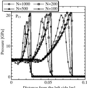
Fig. 4 Pressure profiles along TNT slab (N=100, 200,

500, 1000).

wall. The TNT is detonated from the left side to the right side along the axial direction. This problem is simulated by Shin and Chisum

¹⁴⁾

using a coupled Lagrangian-Eulerian method and Liu et. al.

¹⁵⁾

using a standard SPH method. In this study, we adopt the C-J volume burn technique as a detonation model. The other parameters for TNT are the same as Shin and Chisum.

Figure 3 shows the pressure profiles obtained from the simulation at 2 µs intervals respectively. The simulation is conducted using 1000 particles and the parameters of the artificial viscosity, a =2.0, b =2.0, h =0.01. The circles show the results of Shin and Chisum using 2000 elements and the horizontal line is the C-J pressure, 21 GPa. The pressure takes a peak value on the detonation front and decreases with the distance from there, smoothly. The pres- sure profiles agree with each other. This simulation result shows that the code is valid for the simulation of the deto- nation of high explosive.

Figure 4 shows the case of the number of particles, N=100, 200, 500, and 1000. The pressure profile becomes bluntly with decreasing the particles. However, the peak pressure converges on the C-J pressure with the progress of time and the profiles roughly show the similar distributions except the lowest number of particles. Therefore, we use the relatively small number of particles in a two-dimension- al simulation to prevent CPU time from increasing.

3.3 Underwater explosion of a cylindrical high explosive

A cylindrical shape is often seen on the use of explosives such as an explosion in a cylindrical pressure vessel. An under water explosion of a cylindrical high explosive is fre- quently used to generate an underwater shock wave. It becomes the basis of other applications and is an example of a cylindrical problem.

The cylindrical high explosive, SEP in this study, sets along an axial direction. The diameter and length are 10 mm and 250 mm respectively. The ambient water zone has to be prepared widely enough not to interact an underwater

shock wave with a boundary. The particles of the high explosive and water are arranged at fixed intervals, dx =0.5 mm, and initially have the values at atmospheric condition.

We cut out the unnecessary water particles from the initial particle arrangement to reduce the total number of particles, so that the outline of the simulation area is not a rectangle.

The axisymmetrical condition is given by using the dummy particles. In addition to these particles, we use the fictitious particles lying between the water particles and the explo- sive particles. The fictitious particles are used to prevent a mixture between the water and the explosive particles and they move with time. An artificial external force similar to the Lennard-Jones one

¹⁶⁾

acts between the fictitious particles and the others, however the fictitious particles aren’t used to approximate physical quantities. The initial smoothing length and the coefficient of artificial viscosity are 1.6 dx, a =3.0, b =2.0, h =0.01 on explosive and 1.6 dx, a =0.5, b

=2.0, h =0.01 on water respectively.

Figure 5 shows the configuration of the underwater shock wave (UWS) and of the boundary between the detonation product gas and water (WB). The triangles and the circles show the result obtained from the past experiment

¹⁷⁾

. The simulation result shows the values at the peak pressure point. Although the difference between the simulation and the experiment is a slight large in the region away from the detonation front, the simulation result almost coincides with the experimental result both the underwater shock wave and the boundary. The difference about the boundary shape near the detonation front is caused by the difficulty in obtaining the boundary shape near the detonation front from the experiment owing to the influence of very strong shock wave.

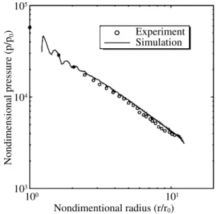
Figure 6 shows the pressure distribution along the under- water shock wave front. The circles and the solid line show the experimental and the simulative result. The radius and pressure are non-dimensionalized by the initial radius of explosive and the atmospheric pressure respectively. Near the detonation front, it is difficult to obtain the peak pres- sure value clearly from the simulation result because of the

80

60

20 40

Radius [mm]

0

Distance from detonation front [mm]

0 100 200

Experiment Simulation

UWS

WB

Fig. 5 Outline of underwater shock wave.

Nondimensional pressure (p/p

0

)

Nondimentional radius (r/r

0

) 10

¹

10

⁰

10

³

10

⁴

10

⁵

Experiment Simulation

Fig. 6 Pressure distribution along underwater shock wave.

complicated situation. Therefore, the pressure profile isn’t clear near the explosive. It shows, however, a good corre- spondence between the simulation and the experiment as a whole. From these results, we think that the particle method is useful for the simulation using explosives though it requires more researches.

4. Conclusion

In this study, we have made the axisymmetrical SPH code based on the MLS method in a cylindrical coordinate sys- tem and have carried out the simulation of an underwater explosion using high explosive to confirm the effectiveness of the particle method.

The simple piston problem shows that the cylindrical code can obtain the same result as that of the standard Cartesian code.

The result of one-dimensional TNT detonation agrees with that of other numerical simulation method. Although it requires the use of a lot of particles to obtain the fine result, the basic profile can be obtained from the comparatively small number of particles.

In the simulation of an underwater explosion, the shock wave front and the boundary between the detonation prod- uct gas and water agree with the result obtained from previ- ous experiment. It also shows the correspondence about the relation between the pressure along the shock wave front and radius.

From these results, we conclude that the particle method is useful for the simulation using explosives. However, we still need further researches.

References

1) S. Itoh, Materials Science Forum, 465-466, 453 (2004).

2) H. Iyama, S. Nagano, and S. Itoh, Sci. Tech. Energetic Materials, 64, 52 (2003).

3) T. Belytschko, Y. Krongauz, D. Organ, M. Fleming, and P.

Krysl, Computer Methods in Applied Mechanics and Engineering, 139, 3 (1996).

4) Li. Shaofan, and W. K. Liu, Applied Mechanics Reviews, 55, 1 (2002).

5) G. A. Dilts, Int. J. Numer. Methods in Engineering, 44, 1115 (1999).

6) G. A. Dilts, Int. J. Numer. Methods in Engineering, 48, 1503 (2000).

7) L. B. Lucy, The astronomical Journal, 87, 1013 (1977).

8) Y. Nadamitsu, M. Fujita, and S. Itoh, Trans. Jpn. Soc. Mech.

Eng., 64B, 1379 (1997), (in Japanese).

9) J. W. Swegle, and S. W. Attaway, Computational Mechanics, 17, 151 (1995).

10) J. J. Monaghan, and R. A. Gingold, J. Comput. Phys., 52, 374 (1983).

11) A. G. Petschek, and L. D. Libersky, J. Comput. Phys., 109, 76 (1993).

12) L. Brookshaw, Australian and New Zealand Industrial and Applied Mechanics Journal, 44, C114 (2003).

13) Y. Nakamura, The Physics of Fluids, 26, 1234 (1983).

14) Y. S. Shin, and J. E. Chisum, Shock and Vibration, 4(1), 1 (1997).

15) G. R. Liu, M. B. Liu, K. Y. Lam, and Z. Zong, Computational. Fluid and Solid Mechanics, 323 (2001).

16) J. J. Monaghan, J. Comput. Phys., 110, 399 (1994).

17) S. Itoh, A. Kira, Y. Nadamitsu, S. Nagano, M. Fujita, and T.

Honda, Trans. Jpn. Soc. Mech. Eng., 63B, 2349 (1997), (in Japanese).