)1(m)-(yk (y) L

Development of new loss function based on Taguchi’s method- Improved Taguchi loss function

Mohammad Abdolshah

Engineering Faculty, Islamic Azad University, Semnan Branch, P.O. Box 35136-93688, Semnan, Iran [email protected]

Abstract: Loss functions are used widely to predict the quality losses and also for various purposes such as manufacturing and environmental risks, decision-making, quality engineering, tolerances design and capability analysis. In this paper first we analyze the weak points of main quality loss functions such as Taguchi loss function, Ryan loss function, inverted normal loss function, asymmetric inverted normal loss function and revised inverted normal loss function and then we propose a new loss function which is called improved Taguchi loss function (ITLF). This new loss function is asymmetric, bounded and reasonable function and also is more realistic compared to the other functions. Finally an example was used to ITLF compare with other loss functions.

[Mohammad Abdolshah. Development of new loss function based on Taguchi’s method- Improved Taguchi loss function. Academ Arena 2017;9(9):87-92]. ISSN 1553-992X (print); ISSN 2158-771X (online).

http://www.sciencepub.net/academia. 9. doi:10.7537/marsaaj090917.09.

Keywords: Improved Taguchi loss function, Taguchi loss function, asymmetric, bounded, quality loss function

1. Introduction

In today’s competitive business environment, it is becoming more and more important for companies to evaluate and minimize their losses. Loss functions have been widely used for several decades. These functions were not only used widely to predict the losses but also for various purposes such as evaluating manufacturing and environmental risks (Pan, 2007), decision-making (Kethley, 2008; Batsony and Shishooy, 2004; Chen, 2004; Wang and Chen, 1999), quality engineering (Shu et al, 2006), tolerances design (Naidu, 2008; Chen, 1999; Feng et al, 2006) and capability analysis (Hsieh and Tong, 2006). There are different forms of loss functions such as squared error, absolute error, weighted and binary loss. Each of these forms tacitly assumes that the larger the error in estimating parameter values the larger the losses will be incurred (Leung and Spiring, 2004).

One of the most well-known loss functions is Taguchi loss function which has been proposed by Taguchi (1986). This function is a quadratic function which primarily has been successfully applied in some areas of quality control and also to other fields. The concept of Taguchi’s (1986) quadratic quality loss function was based on measuring the cost of customers if the product quality is far from the target value.

Moreover there are some other loss functions such as Ryan loss function (Ryan, 1989), inverted normal loss function (Spring, 1993), asymmetric inverted normal loss function (Spring, 1998), revised inverted normal loss function (Pan and Wang, 2000).

Each of these loss functions has some weak points, so the objective of this study is to propose a new loss function base on Taguchi loss function which is more applicable and reasonable.

2. Literature Review

Nowadays loss functions have been used vastly in different fields (Amanda et al.,2012; Yang Zhang et al., 2011; Keartisak Sriprateep, 2011; Niao Na Zhang et al., 2011; Qun Cao et al., 2011; Rens van et al.

2012). Genichi Taguchi (1986) developed his methods in loss functions for Japanese companies that were interested to improve their processes in order to implement total quality management. His method prepares a new approach to understanding and interpreting process information. Taguchi assumes the target as a base point and desired aim for all data and, defines losses for all data that have distance with the target. In the other word, Taguchi losses can include accepted products which may cause customer dissatisfaction and loss of company reputation. So Taguchi loss functions (TLF) detect the customer desire to produce products that are more homogeneous. In this approach and in addition to traditional costs of re-work, scrap, warranty and services costs, cost of inhomogeneous will be assumed. Taguchi loss function is as follows:

) 1 ( m)

- (y k (y)

L  ²

Where L (y) is the loss associated with a particular value of quality character y, m is the target value of the specification; k is the loss coefficient, whose value is constant and depends on the cost at the specification limits and the width of the specification.

Taguchi loss function is one of the most well-

known and applicable loss functions that has been

used vastly. Ryan (1989) proposed a loss function

based on Taguchi loss function with assumption a

maximum loss for L (y), and then suggested constant

loss from a specific point (for example from specific limits). In other words, this function is bounded. Ryan loss function was defined as follows:

 

 

) 2 (

2







 

















B T K y if K

B T K y if T

y B y L

Where K is the maximum value of quality loss, B represents the coefficient of quality loss within the specification limits.

Spring (1993) proposed another well known loss function. Because this function uses normal probability density function, it is called inverted normal loss function (INLF). Inverted normal loss function has defined as follows:

   

) 3 2 (

exp

1 ₂

2

 

 



 

 



 





 



 







L

T K y

y

L 

Where K is the maximum loss if the characteristic deviated from the target, and L is the parameter for controlling the shape of loss function depending on the realistic loss. This loss function is unbounded and symmetric function. Because in real world, the loss of two sides are different so, symmetric functions are not applicable functions and asymmetric functions are more reliable. For example regarding to Equation 1 Spring and Yueng (1998) proposed an asymmetric loss function called asymmetric INLF. Asymmetric INLF defines as follows:

 

 

  ^{( 4 )}

exp 2 1

exp 2 1

2 2

2 2

2 1

2 1















 



 



 

 













 







 

 



 

 













 







T y T if

K y

T y T if

K y

y L

L L





Where K 1 is the maximum loss if the characteristic deviated from the target from left side and K 2 is the maximum loss if the characteristic deviated from the target from right side.

The main idea of Taguchi was that when performance of process departs farther away from the target, the customer’s satisfaction will decrease, and for specifications near target, Taguchi loss function, INLF and asymmetric INLF assume losses, while these products with specifications near target are accepted products and can satisfy customer easily. Pan

and Wang (2000) assume a specific acceptable range (L, U) and no loss for products within this range. Thus Pan and Wang (2000) proposed their loss function which is called revised inverted normal loss function (RINLF).

 

 

 





















 

 



 

 













 











 

 



 

 













 







U y U if

K y

U y L if

L y L if

K y

y L

L L

2 2

2 2

2 1

2 1

exp 2 1

) 5 ( 0

exp 2 1





where (L, U) is the acceptable range of a quality characteristic; K 1 is the maximum loss if the characteristic deviates from the target and exceeds the LSL; K 2 the maximum loss if the characteristic deviates from the target and exceeds the USL;

2 L2 2 L ,

1



 are the parameters for controlling the shape of function depending on the realistic loss.

3. Weaknesses of quality loss functions

As mentioned a weak point of Taguchi loss function is that it is unbounded. In many manufacturing processes, it is unrealistic to assume the quality loss is unbounded even if the material, labor and other administrative costs are included (Pan, 2007), for example sometimes because of specification which is very far from the USL or LSL, we have a tremendous and unrealistic loss. So manufacturers cannot use unbounded functions easily.

Among quality loss functions, just Ryan loss function is a boundary loss function.

Another weak point of Taguchi loss function is its symmetric function. There are many manufacturing processes which have separate losses in different sides of targets, for example in the case of machining process for the final dimension of components, if the specification of dimension is more than target or even USL, with re-machining and few costs, the component will be reworked, but if the specification is less than LSL, the component cannot be repaired and is scraped with high costs and losses. Taguchi, Ryan loss function and INLF are symmetric loss functions whereas asymmetric INLF and RINLF are asymmetric functions. Asymmetric quality loss is also common in cases such as the scrap cost is different from the rework cost.

The last weak point of Taguchi loss function is its unreasonable losses. When the quality characteristic falls within the specification limits or a tighter neighborhood of target value, we do not have rejects or at least from the customer’s point of view.

So a good loss function must be reasonable in

depicting the real losses which occur. Among quality loss functions which mentioned, just RINLF has a specific acceptable range (L, U) without loss within this range.

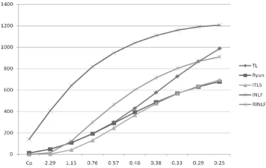
So we can conclude that an appropriate loss function must have three characteristics: boundary, asymmetric and reasonable. In this point of view, we compared the different loss functions in Table 1. In order to overcome the weaknesses of loss functions, a new loss function have been proposed.

Table 1. Comparison of different loss function in point of view of boundary, asymmetric and reasonable Quality loss

functions boundary asymmetric reasonable ¹ Taguchi loss

function

Ryan loss

function 

INLF Asymmetric

INLF 

RINLF  

4. Improved Taguchi loss function (ITLF)

Before Taguchi definition, traditional quality is defined by good or bad. If the specification was within specification limit, the product is good; otherwise it was marked as a reject. But the main idea of Taguchi was that while performance of process departs farther away from the target, the customer’s dissatisfaction

1 - reasonable in depicting the real losses

will increase, and absolutely it cannot be linear, so he suggested a quadratic curve. Sometimes tolerance is tight, and some parts of normal curve remains out of USL or LSL. These parts are rejects and will have extra cost for manufacturer. These parts are kind of loss that create more problems such as detecting, reworking, disposal and bad reputation. These things such as production resources, cost of identification, scrap or rework and liability also have a maximum loss. As a result, the traditional loss function is inadequate to describe the loss associated with a product characteristic. So we propose ITLF, which scrape parts, greater coefficient will be assumed.

) 6 (

/ / T)

- (y k

T) - (y k

0 T) - (y k

/ T)

- (y k

/

(y) ITLF

2 1 4

2 1 2

2 1 1

2 1 3



























































B K T T y B

LSL y B K T

L y LSL

U y L

USL y U

B K T y USL

B K T y A

B B

A A

Where k 1 and k 2 are coefficients which stand for the ordinary loss function for (accepted parts) and k 3

and k 4 stand for the high loss function coefficient (rejects parts). K A is the maximum value of quality loss in left side and B represents the coefficient of quality loss within the specification limits in left side.

Similarly K B is the maximum value of quality loss in right side and A represents the coefficient of quality loss within the specification limits in right side.

Figure 1. Improved Taguchi loss function T  K _A / B B

K

T  _B /

The improved Taguchi loss function has shown in Figure 1. This loss function has bellow features:

1- Regarding to higher loss of reject parts (such as detecting, reworking, disposal and bad reputation cost), the coefficient for data specification which are more than USL and less than LSL is more than normal specification within specification limits. So these losses are more realistic.

2- Since ITLF, has limited the maximum loss to K A and K B , this loss function is bounded and more applicable in industries.

3- Since the amount of losses within the range (L, U) is zero, this function is more reasonable compared with other loss function such as Taguchi loss function, Ryan loss function and INLF.

4- Since ITLF use different coefficient such as k 1 , k 2 , k 3 and k 4 in both sides, so another feature of this function is its asymmetric function.

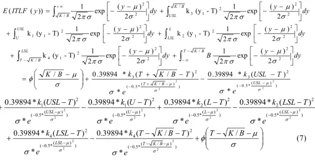
5- The expected value of improved Taguchi loss function is:

y dy y dy

y ITLF

E ^{K B}

USL B

K 





 

 



 





 

 



  ^{ }  ²

/ 2

2 1 2 3

2

/ 2

) exp (

2 T) 1 - (y 2 k

) exp (

2 )) 1

(

( 





 







y dy

y dy

^L

LSL USL

U







 

 



 





 

 



  

²

2 2

1 2 2

2 2

1

1

2

) exp (

2 T) 1 - (y 2 k

) exp (

2 T) 1 - (y

k 





 







y dy B

y dy ^{T K B}

LSL B K

T 





 

 



 





 

 



      ^ 2

/ 2 2

2 /

2 1

4 2

) exp (

2 1 2

) exp (

2 T) 1 - (y

k 





 







) )

* ( 5 . 0 (

2 3

) ) /

* ( 5 . 0 (

2 3

2 2 2

2

*

) (

* 39894 . 0

*

) / (

* 39894 . 0 /









 



  _

 

 

 



 

 





 



 

 T K B USL

e

T USL k e

T B K T k B

K

) )

* ( 5 . 0 (

2 2

) )

* ( 5 . 0 (

2 2

) )

* ( 5 . 0 (

2 1

) )

* ( 5 . 0 (

2 1

2 2 2

2 2

2 2

2

*

) (

* 39894 . 0

*

) (

* 39894 . 0

*

) (

* 39894 . 0

*

) (

* 39894 . 0

























 

 

 

 

 

 

 

 

LSL L

U USL

e

T LSL k e

T L k e

T U k e

T USL k

) 7 / (

*

) / (

* 39894 . 0

*

) (

* 39894 . 0

) ) /

* ( 5 . 0 (

2 4

) )

* ( 5 . 0 (

2 4

2 2 2

2

 





 



  

 

 

 



 

  

 

  ^







B K T e

T B K T k e

T LSL k

B K LSL T

5. Numerical example

Now in order to clarify and explain the improved Taguchi loss function, we can compare this function with other loss functions. For this aim, we compare 10 samples with different standard deviation and same target, USL, LSL and  . Assume our samples have

normal distribution with   122 . 5 . Customer specifications are USL=136.5, Target= 122.5 and LSL=109. Other relevant coefficients are k 1 =2, k 2 =2.5, k 3 =4, k 4 =4.5, A=3, B=4, K A =K B =1600, Δ=3.4375 and for RINLF, k 1 =k 2 =1600. For these samples standard deviation will vary from 2 to 20.

Table 2. Comparison of different loss functions with ITLS

ID Sigma T USL LSL Cp TLF Ryan ITLS INLF RINLF

1 2 123 137 109 2.29 12.00 12.00 0.00 139.41 0.00

2 4 123 137 109 1.15 48.00 48.00 3.45 407.43 13.84

3 6 123 137 109 0.76 108.00 108.20 42.54 643.82 125.85

4 8 123 137 109 0.57 192.00 192.30 131.49 819.28 298.06

5 10 123 137 109 0.46 299.93 291.86 247.07 946.79 463.73

6 12 123 137 109 0.38 430.47 393.56 365.93 1040.88 603.53

7 14 123 137 109 0.33 577.16 487.47 474.81 1110.62 716.12

8 16 123 137 109 0.29 727.35 567.69 567.23 1160.32 803.35

9 18 123 137 109 0.25 867.44 631.59 640.69 1192.22 867.47

10 20 123 137 109 0.23 988.03 679.05 695.47 1208.47 911.28

As shown in Table 2, while standard deviation is increasing, process capability C p is decreasing from 2.29 to 0.23. As process capability decreases, there will be more increase in the rate of rejects and

reworks (losses). So the behaviors of different loss functions are shown in Figure 2. Among all loss functions, it is obvious that in capable process with C p

more than 0.76 the ITLS is less than all, because this

loss function is more realistic and reject- based. For not capable process with C p less than 0.76 this loss

function has an accelerating increasing rate that shows its high sensitivity to major losses.

Figure 2. Comparison of different loss functions with ITLS 6. Conclusion

There are many loss functions such as Taguchi loss function, Ryan loss function, INLF, Asymmetric INLF and RINLF which are used in many different fields. Most of these functions are not boundary or asymmetric functions. Also because of special attitude about departure from mean, they cannot separate real losses (scrapes and reworks). In other words as shown there is no loss function which is boundary, asymmetric and reasonable. So a new loss function called ITLS was developed based on Taguchi method.

ITLS is boundary, asymmetric, reasonable and applicable. As it shown in numerical example ITLS is more realistic and prepares a better meaning of loss in a process. So with the aid of this loss function, manufacturers will be able to depict their real losses.

Corresponding Author:

Dr. Mohammad Abdolshah Faculty of engineering

Islamic Azad University, Semnan Branch, E-mail: [email protected]

References

1. Batsony R. G. and Shishooy S., (2004), Algorithm for optimal loss reduction in serial manufacturing, Int. J. Prod. Res., Vol. 42, no. 5, 883–899.

2. Chen C. H., (1999), Specification limit under a quality loss function, Journal of Applied Statistics, Vol. 26, No. 8, 903- 908.

3. Chen C. H., (2004), Determining the Optimum Process Mean of a One-sided Specification Limit with the Linear Quality Loss Function of Product, Journal of Applied Statistics, Vol. 31, No. 6, 693–703 .

4. Feng, Qianmei and Kapur, Kailash C. (2006) 'Economic development of specifications for 100% inspection based on asymmetric quality loss functions', IIE Transactions, 38:8,659 – 669.

5. Hsieh K. L., Tong L. I., (2006), Incorporating process capability index and quality loss function into analyzing, the process capability for qualitative data, Int J Adv Manuf Technol 27:

1217–1222.

6. Kethley R. Bryan, (2008), Using Taguchi Loss Functions to Develop a Single Objective Function in a Multi-Criteria Context: A Scheduling Example, International Journal of Information and Management Sciences Volume 19, Number 4, pp. 589-600.

7. Leung, B.P.K. and Spiring, F.A. (2004), Some properties of the family of inverted probability loss functions, Quality Technology and Quantitative Management, Vol. 1 No. 1, pp. 125- 47.

8. Naidu N.V.R. (2008), Mathematical model for quality cost optimization, Robotics and Computer-Integrated Manufacturing 24 811–

815.

9. Pan J. N. and Wang J. H., (2000), “A Study of

Loss Functions for Product Interference

Analysis”, Industrial Engineering Research, vol.

2(1), pp. 80-100.

10. Pan J. N., (2007), A new loss function-based method for evaluating manufacturing and environmental risks, International Journal of Quality & Reliability Management Vol. 24 No.

8, pp. 861-887.

11. Ryan T. P., (1989), Statistical Methods for Quality Improvement, Wiley, New York.

12. Shu M.H., Wang Chih-Hsiung, Hsu B.M., (2006), A review and extensions of sample size determination for estimating process precision and loss with a designated accuracy ratio, Int J Adv Manuf Technol 27: 1038–1046.

13. Spring F. A. and Yueng A. S., (1998), “A General Class of Loss Functions with Industrial Applications,” Journal of Quality Technology, vol. 30(2), pp. 152-162.

14. Spring F. A., (1993), “The Reflected Normal Loss Function,” The Canadian Journal of Statistics, vol 21, pp. 321-330.

15. Taguchi G., (1986), Introduction to Quality Engineering: Designing Quality Into Products and Processes, Asian Productivity Organization, Tokyo.

16. Wang R. C. and Chen C. H., (1999) Designing a variable sampling plan based on Taguchi’s loss

function, Journal of Applied Statistics, Vol. 26, No. 3, 309- 313.

17. Rens van de Schoot, Herbert Hoijtinka, Jan- Willem Romeijnd, Daniel Brugman, (2012), A prior predictive loss function for the evaluation of inequality constrained hypotheses, In press.

18. Amanda J. Schmitt, Lawrence V. Snyder, (2012), Infinite-horizon models for inventory control under yield uncertainty and disruptions, Computers & Operations Research, Volume 39, Issue 4, Pages 850-862.

19. Yang Zhang et al., Application of Cluster Analysis and Trend Extraction in Wind Speed Series Consistency Correction, (2011), Applied Mechanics and Materials, 130-134, 3425.

20. Keartisak Sriprateep, (2011), Optimization for Turning Metal Matrix Composites with Multiple Performance Characteristics, Applied Mechanics and Materials, 121-126, 1479.

21. Niao Na Zhang et al., (2011), The End-Point Ingredient Prediction of Low Carbon Ferrochrome Smelt Based on the Working Condition, Applied Mechanics and Materials, 128-129, 1246.

22. Qun Cao et al., (2011), Forecasting Model Based on SAGA and LS-SVM for the Water Quality of Poyang Lake, Advanced Materials Research, 347-353, 781.

9/25/2017