Learning from Cluster Examples

Learning from Cluster Examples

KAMISHIMA, Toshihiro

Doctor Thesis of Informatics, Kyoto University

2001

Abstract

Learning from cluster examples (LCE) is a hybrid task combining features of two com- mon classification tasks: clustering and learning from examples. In LCE, each example is an object set with the true partition for the set, where the true partition is the one that users consider as the most appropriate for their aim among the possible partitions. The task is then to acquire a rule for partitioning unseen object sets from this example set. A method for learning such partitioning rules is useful in any situation where explicit al- gorithms for deriving partitions are hard to formalize, but where individual examples of true partitions are easy to specify. Clustering techniques have been of necessity applied to such situations, despite being essentially unsuited to the problems. We point out faults in using clustering techniques under such a situation, and explain why the techniques for LCE task expected to be overcome these faults. We then present a solution technique for LCE task, and apply the method to the problems in two domains; one with dot patterns and the other with more realistic vector-data images.

i

Contents

1 Introduction 1

2 An Overview of Learning from Cluster Examples 3

2.1 Why LCE Is Important . . . . 5

3 Formalization of Learning from Cluster Examples 13

3.1 Notes on The Formalization of LCE . . . . 16

4 The Partitioning Method 21

4.1 How To Maximize The Probability: Pr[π=π

; {A(o)} , {A(p)}] . . . . . 25

5 The Learning Methods 33

5.1 Acquisition of The Function: f

(p) . . . . 33 5.1.1 Our Algorithm to Estimate The Function: f

(p) . . . . 35 5.2 Acquisition of The Function: f

(A(π)) . . . . 40

6 Experimental Domains and Testing Methods 47

6.1 Experimental Domains: Dot Patterns . . . . 47

iii

6.1.1 Attributes for Dot Patterns . . . . 51

6.2 Experimental Domains: Vector-data Images . . . . 55

6.2.1 Attributes for Vector-Data Images . . . . 58

6.3 A Testing Method . . . . 61

7 Experimental Results and Discussions 65 7.1 Testing Using Dot Patterns . . . . 66

7.2 Testing Using Vector-data Images . . . . 81

7.3 Discussions . . . . 86

8 Conclusions 89

A The Description Length for the Decision Lists and Example Sets 91

Chapter 1

Introduction

Clustering is a typical task that involves partitioning a given object set into subsets whose constituents are mutually similar. Since clustering is carried out based on rules or criteria given in advance, it can be regarded as deductive technique for partitioning.

In this paper, we advocate the use of an inductive technique for partitioning. In other words, we try to acquire a partitioning rule from an example set consisting of pairs of an object set and the true partition for the object set, where the true partition is the one that users consider as the most appropriate for their aim among the possible partitions.

The acquired rule can then be used for finding the true partitions for unseen object sets (not appearing in the example set). Our induction task is similar to that of learning from examples, that acquires a rule for classification from a given example set, except that an aim of our task is to acquire a rule not for classification but for partitioning. Since our learning task also deal with partitioning like a clustering task, we give our new task the

1

composite name learning from cluster examples, or LCE.

A solution technique for LCE will be useful for any problem where users can easily identify which partition is the true partition for a given object set, but cannot specify explicit rules for deriving these partitions. No technique that has been developed for this aim. To fill the void, clustering techniques have been of necessity used, but they are not particularly suited to such kinds of partitioning. In this paper, we point out several faults caused by applying clustering techniques to such problems, and explain how our techniques are expected to overcome these faults.

We experimentally apply our technique to the problems for partitioning two types of data. We apply the method to the problems in two domains; one with dot patterns and the other with more realistic vector-data images. Since there are no other algorithms designed specifically for the tasks we consider, we cannot show direct comparison results.

Therefore we pay particular attention to confirming whether our LCE algorithm has ability to acquire useful rules, and to analyzing the behavior of our method.

We proceed as follows. In Chapter 2, we show the importance of the LCE task. In

Chapter 3, we formalize the problem. In Chapter 4 and 5, we then present partitioning

and learning methods respectively. In Chapter 6, we explain experimental domains and

a testing method. In Chapter 7, we show results and discuss them. Finally, Chapter 8

summarizes our conclusions.

Chapter 2

An Overview of Learning from Cluster Examples

In this chapter, we first present an overview of the LCE task, and then explain importance of the LCE task.

LCE is a composite task combining features from the techniques of clustering and of learning from examples. To give an overview of LCE, we therefore begin by reviewing these existing tasks.

Learning from examples is a task involving the acquisition of a rule for classification from a given example set. Each example is a pair of an object and a class to which the object should belong. The acquired rule is used to classify an unseen object into a proper class. The typical technique for this task in the machine learning field is ID3 [20] or feed- forward neural networks [2], and the task is often called discriminant analysis or pattern

3

recognition.

Clustering, on the other hand, is a task that partitions a given object set into clusters that have the properties of internal cohesion and external isolation [7]. The minimum distance or the k-means is a typical clustering method in the numerical taxonomy litera- ture. In the machine learning literature, the task is often called learning by observation or unsupervised learning. COBWEB [8] and AutoClass [5] are typical examples of such a

learning algorithm.

We have been developing “learning from cluster examples” techniques [12] as an

extension of these two known approaches. The aim is not to find a rule to classify single

objects, or a particular clustering, but to find a rule for partitioning, based on a given

example set. Each example is a pair of an object set and an instance of the true partition

for the object set. Note that, the true partition is the one that users consider as the most

appropriate for their aim or intention. The acquired rule produced by learning from this

example set is used to derive the true partition for an unseen object set. So, in contrast to

learning from examples, LCE involves the acquisition of a rule not for classification but

for partitioning an object set. And whereas the aim of clustering is to partition an object

set based on rules or criteria given in advance, the aim of LCE is acquiring partitioning

rule, that can be applied to any object set from the same domain. In short, LCE takes the

inductive nature of learning from examples, and brings it to the task of clustering.

2.1. WHY LCE IS IMPORTANT 5

2.1 Why LCE Is Important

We will now describe some example cases which fit for the LCE task. Typically, these will be cases where an true partition for any object set is easy for a user to specify or identify, but where an overall set of rules for finding these partitions is very hard for a user to specify concretely and explicitly. A prime example of such a problem is image segmentation. Suetens et al [27] quoted Kanade’s view of the segmentation problem, that is to obtain a segmentation which separates out semantically meaningful objects or parts of objects.

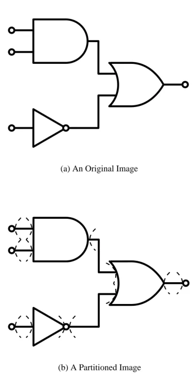
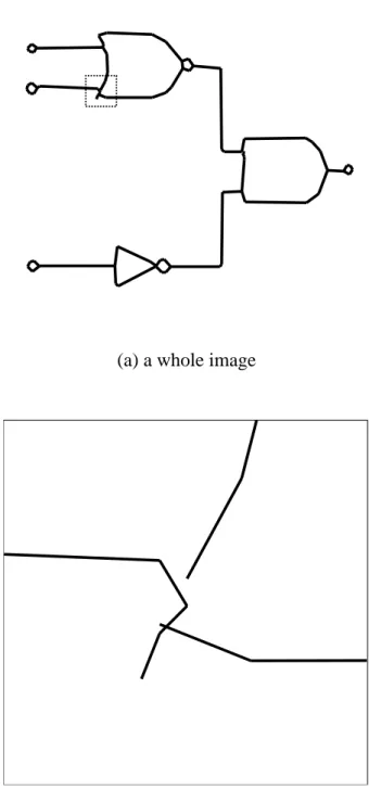
To explain the image segmentation task, we give an example of a typical problem

involving the understanding of diagrammatic images. Figure 2.1(a) shows an image of

a logic circuit diagram. Understanding this image is to obtain a proper description of

the form of its logic circuit. In this case, a proper description for the image would be

the logic function “a · b + ¯ c.” In a typical diagram image understanding process, the

given image is first of all partitioned, so that each cluster depicts an individual primitive

symbol. This partitioning operation is generally called segmentation in the machine vision

literature and is a very common technique. An appropriate treatment of the image in

Figure 2.1(a), for example, would be to partition it into clusters with each depicting one

part of a logic circuit diagram. Such a partition is illustrated in Figure 2.1(b), where the

the original image has been separated with thin broken lines. After segmentation, each

cluster is mapped to its proper primitive symbol. From the set of mapped symbols, an

image description can then be inferred.

(a) An Original Image

(b) A Partitioned Image

Figure 2.1: Examples of diagram images

2.1. WHY LCE IS IMPORTANT 7 Segmentation is needed in many types of image understanding processes. As in the example we gave above, it typically corresponds to the task of finding partitions that satisfy the users’ aims in situations where the users themselves cannot specify general rules for deriving partitions. Although segmentation problems are frequently encountered, we don’t know methods that squarely grapples with the problem. Image segmentation techniques, for example, are usually designed in a non-systematic manner, relying on the designers’ experience and intuition. Though such a design approach has been used from the beginning of machine vision research, the resulting programs are usually restricted to processing images in limited domains. We can pinpoint a number of drawbacks that arise from this absence of a systematic approach:

• Segmentation methods commonly rely on the designers’ intuition. An example

of a successful image understanding process is OCR (Optical Character Reader)

systems. These systems are capable of recognizing regions where characters are

written in a given document image. For this specific purpose, the powerful segmen-

tation technique XY-Tree [9] was developed. This exploits a very specific feature

of document image analysis: there are always gaps between lines or between char-

acters. Another example of structure in a domain is RoboCup [14], in which soccer

games are played by AI-controlled robots. These robots have to use machine vision

to understand the game, but structure is artificially introduced by using distinct col-

ors to identify objects. For example, the ball is orange and the goals are either blue

or yellow. These coloring regulations are a significant aid that the robots attempts

to locate objects.

In cases like these two examples, human designers can state rules describing how images should be partitioned by using image features. In practice, character regions can be extracted by finding gaps between lines or characters in document images, and robots can almost always detect a ball by locating an orange region in the camera image. However, this kind of feature is not common. For example, Minoh et al have worked on the segmentation of line-drawing images, in which structure is hard to find [17]. This work succeeded in extracting symbol candidates from line-drawing images by defining a set of complicated rules for the extraction of symbols in terms of groups of short line-segments surrounded by a loop. This rule was intuitively derived based on a great deal of knowledge regarding the domain of line-drawing images, properties of image processing and cognitive science. In order to find suitable rules in domains where there is no obvious and constant features, the designers have nothing but to rely on intuition in addition to very much effort and knowledge.

• Some features are hard to formalize in pragmatic domains. The features, adopted

in the above successful domains, are usually obvious, and is relatively easy to be

represented by formal rules. We call such types of features typical features. How-

ever, there exists unexpected and ambiguous features that have to be taken into

account for segmentation. We call them exceptional features. We give an example

of exceptional features in the above Minoh’s work. It is a very frequent event that

2.1. WHY LCE IS IMPORTANT 9 a surrounding loop happens to be cut, and extraction of symbols will be failed by this event. Such events can be often caused, for example, by stains on an original diagram, quantization errors in scanning, or the effects of image processing. The designers therefore have to take into account these events, but it is not easy to iden- tify the features that how and where these events will occur. Such features are just what we call exceptional features. (In Section 6.2, we give some practical examples of such features). In a pragmatic domain, even though designers notice that these events will occur and try to formalize the features of the events, it is difficult to formalize such features as concrete rules by hand.

• Segmentation rules require user tuning. The designers of a system will create rules that express the typical features of the input, but these features will almost always allow for some variation. Since the nature of these variations are too difficult to cap- ture intuitively, designers usually have no choice but to leave adjustable elements in segmentation rules. When applying a segmentation rule to a new image, experience and knowledge of machine vision is required for the users of the rules. For example, Minoh’s work on image segmentation requests users to specify a threshold value to judge the shortness of the line-segments. Thus users without experience of machine vision techniques will not able to apply these rules.

• Segmentation results are statistically instable. We will show two reasons for this.

Firstly, it is difficult to enforce a strict distinction between training and testing ex-

amples, because partitioning rules are typically created by hand. The designers

will naturally seek to find the best segmentation rules by referring to not only their knowledges of domain but also to available images. Thus, if the human designers just glancing the test images, they unwillingly gain some information from these images. Thus, since it is not avoidable to essentially distinct testing and training images, the performance for unseen images will not be objectively and rigorously evaluated. This facts weaken statistical stability of results derived by acquired rules by hand.

Secondly, an amount of information used for generating partitioning rules is re- stricted. Even though thousands or millions of images are available, the designers can merely deal with restricted amount of information due to the limitation of hu- man cognitive ability. This fact also lead to statistical instability.

Other drawbacks have also been noted by Pavlidis, who pointed out the difficulties in finding partitioning when using several kinds of image features [19]. We believe that the only way to counter all these drawbacks is abandoning the non-systematic design approach in favor of a more powerful general method. Our choice for this method is a design approach based on LCE.

LCE expected to overcome the above drawbacks of existing approaches as follows:

• With LCE the designers only have to provide instances of partitions; it is not re-

quired to explicitly identify features important for segmentation by depending on

their intuition.

2.1. WHY LCE IS IMPORTANT 11

• A learning algorithm can acquire rules that fully represent the domain. By anal- ogy with learning algorithms for the object classification task, we can also see that LCE should handle exceptional features. In object classification, attribute values assigned to objects are often changed by accident, yet algorithm for learning from examples can still acquire successful classification rules. We are confident that a similar approach (that is, acquiring a rule with stochastic techniques from an exam- ple set) will also be effective for acquiring rules for partitioning.

• Just as object classification algorithms can generate rules that can cope with vari- ance in the input, LCE can generate segmentation rules that users will not need to tune, and thus knowledge of machine learning or of the domain is not required when applying rules.

• Finally, since the learning algorithms explicitly require a set of training examples and can be effectively isolated from exposure to the testing examples, performance can be fairly evaluated. Since segmentation rules are acquired not by hand but by statistical algorithms, an amount of information gained from a given examples are not restricted by human cognitive ability any longer. These two property enhance statistical stability.

The development of successful techniques for learning from cluster examples will

contribute to the progress of research in any field involving the mapping of raw sensor

signals to abstract notions of objects. We have discussed a number of example domains

already, and the technique may also be applicable to problems such as multistrategy learn-

ing [16], the data mining [1] and the identification of genes in DNAs [4]. The rest of this

paper will therefore rise to this challenge by presenting our algorithm for LCE.

Chapter 3

Formalization of Learning from Cluster Examples

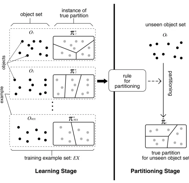
This chapter formally states the task of learning from cluster examples. This task can be visualized as in Figure 3.1 and consists of two major stages: a learning stage and a partitioning stage. In the learning stage (Figure 3.1, left), the rule for carrying out partitioning is acquired from an example set. The example set, EX, includes #EX elements, {(O

, π

) , (O

, π

) , . . . , (O

, π

)}, where O

is an object set and π

is an instance of its true partition. The object set O includes #O elements, {o

, o

, . . . , o

}. The cluster C

is a subset of O, and the partition is a set of these clusters with #π elements, {C

, C

, . . . , C

}, such that the clusters are disjointed and every object has to be an element of exactly one of the C

’s. In the partitioning stage (Figure 3.1, right), based on the acquired rule, the true partition of an unseen object set, O

, is estimated.

13

! #"%$

π

+-,

π

021

π

56798:;=<>? @ABCEDAFGHI

JKLMNOPRQESTQESUV

W

XY[Z\

]_^

`abcd

e`

fhg

i[jk

lmlmnomo

p

qrst

uvw

xyzR{|}{|~|€

π

ƒ„…††‡ˆ‰ŠŒ‹Ž=‘

’E“”•–—˜R™EšT™Eš›œ

EžŸ ¡¢££¤¥¦§Œ¨©ª=«¬­

Figure 3.1: An illustration of learning from cluster examples

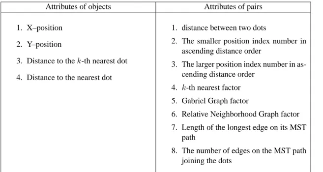
15 Because many of the algorithms used in techniques for learning from examples adopt attribute vectors to represent the individual objects, we also adopt them to represent the individual object set. We introduce the following three types of attributes assigned to different parts of the object set.

Attributes of Objects This type of attribute is assigned to constituent objects. For ex-

ample, the positions of objects can be represented. We denote the attributes of the object o by A(o). A(o) is a vector with #A(o) values, (a

(o), a

(o), . . . ,a

(o)).

Attributes of Pairs This type of attribute is assigned to pairs of constituent objects. For

example, the distances between object pairs can be represented. Specifically, let a pair of objects o

and o

be denoted by p

, and let P be the set of all possible pairs of objects. Thus, P has #O(#O + 1)/2 elements, and this number is denoted by

#P . We denote the attributes of the object pair p by A(p). A(p) is a vector with

#A(p) values, (a

(p) , a

(p) , . . . , a

(p)).

Attributes of Partitions This type of attribute represents characteristics of entire parti-

tions. For example, the number of clusters can be represented. While values of the

above two types of attributes are rely on only an given object set, those of partitions

are not. Given a partition, values of attributes of partitions are calculated from val-

ues of the above two types of attributes and from a states of the partition. When O

is divided into a partition, π, we denote this type of attribute by A(π). A(π) is a

vector with #A(π) values, (a

(π) , a

(π) , . . . , a

(π)).

To apply our learning algorithm, the domains of attributes of objects and of pairs are either continuous numbers or discrete values (as in Quinlan’s ID3 [20]). Also, the domains of attributes of partitions are real numbers from the interval [0 , 1].

3.1 Notes on The Formalization of LCE

We add here two notes relevant to the above formalization.

Firstly, though either attributes of objects or those of pairs are adopted to represent object sets when applying traditional clustering techniques, we adopt both types of at- tributes together in our formalization of the LCE task. Below we describe the reason why both types of attributes are adopted.

It is helpful to sort out partitioning tasks before showing explanation of the above reason. We suppose that the partitioning tasks can be classified into two categories, and call each of these class finding and true clustering respectively.

In the case of the class finding task, objects are independently generated from a pop-

ulation according to an identical distribution, and these generated objects compose an

object set. In the population, there is a set of classes, and each object belongs to one of

the classes. One can observe object sets themselves, but cannot do classes of the con-

stituent objects. An aim of the task is to partition a given object set into clusters, each

of which consists of objects belonging to the same unobserved class. For finding the true

partition, it is therefore enough to investigate relations between features of each object

and class properties. On the other hand, in the case of true clustering task, object sets are

3.1. NOTES ON THE FORMALIZATION OF LCE 17 generated as a group. Constituent objects are not independent any longer, and the true partition is determined based on properties of entire the object set. Therefore, to derive the true partition, mutual influences among the objects have to be taken into account.

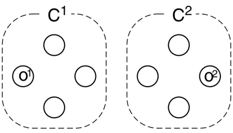
The following phenomenon clarify the difference between these two types of tasks.

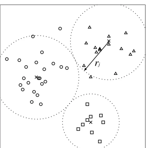
Figure 3.2(a) shows an object set O

that is generated from a population (objects are represented by circles). The true partition for the set consists of two clusters, C

and C

, each of which is depicted by a surrounding broken line. Objects, o

and o

, belong to clusters, C

and C

, respectively. Consider then another object set, O

(shown in Figure 3.2(b)), that is identical except for the object, o

. The object set is also generated from the same population. Examining the true partition for the set O

reveal distinction of two types of partitioning tasks. In the case of the class finding task, o

and o

are sure to belong to different clusters even in the O

. Because objects are generated independently, the existence of the object o

will not affect weather o

and o

are in the same cluster or not. In the case of the true clustering task, these two objects might belong to the same cluster. This is because the mutual influences between the o

and the other objects might completely change the true partition for O

.

To accomplish the class finding task, referring attributes of objects is sufficient for

finding relations between individual objects and the unobserved classes. Therefore clus-

tering techniques that only based on attributes of objects can be regarded as being de-

signed for the class finding task. We may say that some of the clustering or unsupervised

learning techniques, such as k-means or the AutoClass, are classified into this type of

(a) an object set, O

, for which the true partition consists of two clusters.

(b) an object set, O

, that is identical to the above set except for the object, o

Figure 3.2: Two examples of object sets to explain distinction between two types of par-

titioning tasks

3.1. NOTES ON THE FORMALIZATION OF LCE 19 clustering tasks. In contrast, to carry out the true clustering task, it is required to refer mutual influences among objects. So attributes representing features of such influences, i.e. attributes of pairs, is required. The so-called natural clustering tasks or the image segmentation tasks are typical examples. Clustering techniques that can handle attributes of pairs can be regarded as being designed for this type of task, and the minimum distance method is a representative of such techniques.

If a LCE technique can only deal with either of the two tasks, users have to specify which types of tasks they try to solve. Thus we consider that it is required to define LCE formalization that can acquire rules to applicable to the above both types of tasks. It is the reason that we employ both types of attributes together.

We then mention about using attributes of partitions. To derive the true partitions, one

has to take into consideration not only the local features of object sets but also global

features, i.e. attributes of partitions. For example, the attribute “the numbers of clusters”,

is typical example of such global features. To solve the image segmentation problem,

it is required that proper numbers of clusters have to be specified automatically. If LCE

techniques cannot deal with such global features, one will not able to apply the techniques

to solve the segmentation problem. Therefore, we introduced attributes of partitions to our

LCE formalization.

Chapter 4

The Partitioning Method

In this chapter, we describe our partitioning methods. In general, a partitioning rule is firstly learned and then the rule is applied for partitioning, but we describe partitioning method in this chapter for convenience of explanation.

Let π be an arbitrary partition for an unseen object set O, and π=π

be the event that the π is equals to the true partition π

. To select the most plausible true partition among possible partitions, we adopt a maximum a posteriori (MAP) estimator, namely, the one that maximizes the joint probability of an event π=π

and all the attribute value vectors assigned to the object set. The joint probability is

Pr[π=π

, A(π); {A(o)} , {A(p)}], (4.1)

where {A(o)} and {A(p)} are sets of all attribute value vectors assigned to constituents of O and P , respectively. Since {A(o)} and {A(p)} only depend on the given object

21

set and are independent from selection of π, we treat these value vectors as precondition to determine a distribution of the joint probability. Equation (4.1) is hard to calculate directly because a number of elements (#O+#P +1) is not constant, and this property is not suitable for most of statistical techniques. We therefore decompose it into the product of two terms and try to calculate each individually:

Pr[π=π

; {A(o)} , {A(p)}] , (4.2) Pr[A(π)|π=π

; {A(o)} , {A(p)}]. (4.3)

Maximizing the product of these two equations is the key to our method. To maximize Equation (4.2), we show how it can be manipulated into a more manageable form. The details of this manipulation are complicated and we defer them until the next section.

Without going into the details of the representation here, the rewritten equation looks like:

Y

p∈P⁺

f

(p) × Y

p∈P⁻

f ¯

(p). (4.4)

As for Equation (4.3), we make the assumption that it is free from the preconditions {A(o)} and {A(p)}. By definition, the value vector A(π) is calculated from the vectors, {A(o)} and {A(p)}, together with states of a partition, π. Therefore, the effects of {A(o)}

and {A(p)} are already embedded in A(π), even if we didn’t explicitly refer to them as

23 function preconditions. By introducing the assumption, Equation (4.3) is rewritten simply as the probability density:

Pr[A(π)|π=π

]. (4.5)

This density is calculated by the function f

(A(π)), which is acquired by the learning method described in Section 5.2. Consequently, to maximize Equation (4.1), all that we need to do is to maximize the product of Equation (4.4) and Equation (4.5).

We then describe our procedure to search for the most plausible true partition, that is achieving the maximum of the above product. According to the literature (e.g., [7]), the number of possible partitions for O is

X

j=1

à 1 j!

X

i=0

(−1)

µ j

i

¶ i

! ,

and this number increases exponentially according to the number of objects. Therefore, finding the optimal partition is not tractable in general, and we rely on the greedy search algorithm of Figure 4.1 to find a partition that may be locally optimal. In this algorithm, an initial partition is iteratively changed by applying modification operations. In each iteration, the operation that maximize the product of Equation (4.4) and (4.5) is applied.

This iteration stops when no operation improves the product.

The details of this algorithm is as follows. In Figure 4.1, Eq4(π) and Eq5(π) denote

the values of Equation (4.4) and (4.5) when O is partitioned into π, respectively. The algo-

rithm begins by creating an initial partition whose constituent clusters are made up of only

the procedure MAIN

t:= 0,π⁰:={C ={o}, ^∀o∈O}

if (Eq5(π

f :=true,E⁰ :=

Eq5(π

Eq4(π

else

f :=false,E⁰ :=

Eq4(π

start:

t:=t+ 1,E^t:=E^t−1

forall (C

)

π⁰ :=π^t−1−C^A−C^B+{C^A∪C^B}, call EVALUATION

(π

)

if (f

forall (C

)

forall (o

)

π⁰ :=π^t−1−C^A−C^B+{C^A− {o}}+{C^B∪ {o}}, call EVALUATION

(π

)

} }

if (f

) then goto start output

end

the procedure EVALUATION

(π

) if (f

if (Eq5(π

f :=true,π^t:=π⁰

,

Eq5(π

Eq4(π

else if (Eq4(π

) then

π^t:=π⁰

,

Eq4(π

}

else if (Eq5(π

Eq4(π

) then

,

Eq5(π

Eq4(π

return

Figure 4.1: Our algorithm for searching an true partition

4.1. HOW TO MAXIMIZE THE PROBABILITY: PR[π=π

; {A(O)} , {A(P )}] 25 one object, and then refines this partition so as to maximize the product of Equation (4.4) and (4.5). This refinement is done by applying two types of operations: a merge, that merges a pair of clusters, and a move, that moves one element from one cluster to another.

When no partition that achieves a larger value of the product is found, this algorithm stops and then outputs the current partition as the most plausible true partition. Note that, the basic role of the procedure E

is to calculate a value of the product. The value is used to compare two partitions, one is the current, and the other is the one into which the current is transformed by applying arbitrary operations. The E

procedure treats separately the condition, where Equation (4.5) has been zero from the beginning of the algorithm, because the product becomes zero even if a value of Equation (4.4) is non-zero. Therefore, while this condition holds, E

simply returns the value of Equation (4.4), and the moving operation is not applied to avoid infinite loop. Once a partition for which Equation (4.5) is not zero is found, this special case is no longer invoked.

4.1 How To Maximize The Probability:

Pr[π =π ^∗ ; {A(o)} , {A(p)}]

Here we give details on the transformation of Equation (4.2) into Equation (4.4) that we used above.

Because Equation (4.2) refers to many (#O+#P ) value vectors as preconditions and

the number of elements of these vectors is not constant, it is not straightforward to calcu- late its value. Therefore, we adopt the following technique to calculate it. We first gen- erate a set of probabilities each of which is calculated based on two value vectors from {A(o)} and one from {A(p)}. These probabilities are then combined by using Dempster

& Shafer’s rule of combination [26] (DS rule for short). So it is helpful to describe the DS rule before moving on to our calculation method for Equation (4.2).

The DS rule is used for combining probabilities based on different pieces of evidence.

Let e be an event, E

be an event set, and E

be the set of all possible events. Let P (E

) be the power set of E

, i.e. {E

:

E

⊆ E

}. Pr[E

] denotes the probability that one of the events in E

occurs, and is called a basic probability. Basic probabilities satisfy these conditions:

Pr[E

] ≥ 0 , Pr[∅] = 0 , X

Ea∈P(EAll)

Pr[E

] = 1.

Pr[E

; A

] denotes a basic probability for E

based on the evidence A

. Let [E

; A

] be an event set for which Pr [E

; A

] is defined. The difference between [E

; A

] and E

is that the evidence A

is given together or not. Given n distinct pieces of evidences, A

, . . . , A

, an combination of event sets, {[E

; A

] , . . . , [E

; A

]}, is defined as follows.

The [E

; A

] is an arbitrary event set E

∈ P (E

) based on the evidence A

. The rest of event sets are the same as [E

; A

] except for that each of event sets is based on the distinct evidences A

,. . .,A

. The {[E

; A

], . . .,[E

; A

]} is a combination of these event sets. It should be noted that event sets, E

,E

,. . ., E

, may be different or identical. T

{[E

; A

],

4.1. HOW TO MAXIMIZE THE PROBABILITY: PR[π=π

; {A(O)} , {A(P )}] 27 . . . , [E

; A

]} be the intersection of such a combination of event sets. According to the DS rule, the probability of a specific event e based on n evidences is

P

{[E1;A1],...,[En;An]}={e}

³Q Pr[E

; A

]

´

1 − P

T{[E1;A1],...,[En;An]}=∅

³Q Pr[E

; A

]

´. (4.6)

The numerator of the above equation denotes the sum of Q

Pr[E

; A

]’s in the case that T {[E

; A

] , . . . , [E

; A

]} is exactly equal to {e} over the all possible combinations of

event sets. Q

Pr[E

; A

] denotes the product of basic probabilities assigned to [E

; A

] , . . .,[E

; A

] where [E

; A

]’s are the event sets that satisfy the condition of the sum. Con- cretely, consider a combination of event sets {[E

; A

] , . . . , [E

; A

]}. If the intersection of the combination is equal to {e}, a product Q

Pr[E

; A

] is Pr[E

; A

] × Pr[E

; A

] ×

· · · × Pr[E

; A

]. The numerator is the sum of products in all cases that a condition T {[E

; A

] , . . . , [E

; A

]} = {e} is satisfied. The denominator is calculated in the same

way except for summing in the case that the intersection of event sets becomes an empty set.

We then present how to use the DS rule in our transformation of Equation (4.2).

Strictly speaking, the presumptions and semantics of the probabilities manipulated by

the DS and the Bayesian theories are different. However, it is well known that the DS

theory can be regarded as a generalization of the Bayesian theory. Therefore, we intro-

duce the DS theory to calculate the probability of Equation (4.2). Since the precondition

of Equation (4.2) presents an event that sets of attribute value vectors {A(o)} and {A(p)}

are simultaneously observed, by definition, the precondition corresponds to an event that {A(o)} ∪ {A(p)} are observed. This precondition can be treated as evidences in the context of the DS rule, because both of these can be regarded as basis to determine the distribution of π=π

. An overview of the procedure to calculate the probability of Equa- tion (4.2) is as follows: We first extract subsets from {A(o)} ∪ {A(p)} such that the union of the subsets exactly equals to {A(o)} ∪ {A(p)}. We calculate basic probabilities whose evidences are each of the subsets, then combine these probabilities by applying the DS rule. The combined probability can be regarded the probability whose evidence is the attribute value set, {A(o)} ∪ {A(p)}, since the union of the subsets equals to the set itself.

As the subset of value vectors, we choose the subset, {A(o

) ,A(o

) , A(p

)}, that consists of attribute values related to an object pair, p

. Let in(p

, π) be the function that takes 1 if both o

and o

are in the same cluster of the partition π, and 0 otherwise. The following probabilities, f

(p

), are calculated for each object pair in P :

f

(p

) ≡ Pr[in(p

, π

) = 1; A

(p

)],

where π

is the true partition. The attribute A

(p

) is a combination of the three at- tributes, A(o

), A(o

) and A(p

), which we will fully explain in Section 5.1. The function f

(p) is acquired in advance from an example set in the learning stage.

To compute Equation (4.2) by using the DS rule to combine the above probabilities, we first introduce some notations. The function ev(Π) is defined as ev(Π) = {π=π

:

∀

π ∈ Π}, where Π is an arbitrary set of partition. We use Π

to denote the set of

4.1. HOW TO MAXIMIZE THE PROBABILITY: PR[π=π

; {A(O)} , {A(P )}] 29

π¹ =(o¹,o²,o³,o⁴) π² =(o¹)(o²,o³,o⁴) π³ =(o²)(o¹,o³,o⁴) π⁴ =(o³)(o¹,o²,o⁴) π⁵ =(o⁴)(o¹,o²,o³) π⁶ =(o¹,o²)(o³,o⁴) π⁷ =(o¹,o³)(o²,o⁴) π⁸ =(o¹,o⁴)(o²,o³) π⁹ =(o¹)(o²)(o³,o⁴) π¹⁰=(o¹)(o³)(o²,o⁴) π¹¹=(o¹)(o⁴)(o²,o³) π¹²=(o²)(o³)(o¹,o⁴) π¹³=(o²)(o⁴)(o¹,o³) π¹⁴=(o³)(o⁴)(o¹,o²) π¹⁵=(o¹)(o²)(o³)(o⁴)

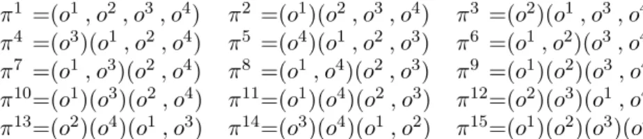
Figure 4.2: An example of all the possible partitions for the object set: {o

, o

, o

, o

} all possible partitions for O. Now, let us focus on the set of basic probabilities whose evidence is A

(p) of an arbitrary p. The function f

(p) can then be rewritten as the following basic probabilities:

 

 

 



Pr[ev(Π(p)); A

(p)] ≡ f

(p), where Π(p) = {π :

π ∈ Π

, in(p , π) = 1}

Pr[ev( ¯ Π(p)); A

(p)] ≡ 1−f

(p), where Π(p) = Π ¯

− Π(p).

To give an example here, consider the object set O = {o

, o

, o

, o

}. For this set,

Π

is the set of fifteen partitions as shown in Figure 4.2, where the objects in parenthesis

form one cluster. And the set Π(p

) is {π

, π

, π

, π

, π

}, since these five partitions

are the only ones which satisfy a condition that o

and o

are in the same cluster. In

general, an event that both objects of p are in the same cluster, by definition, corresponds

directly to an event that O is partitioned into any of the partitions in Π(p). We assign a

probability of zero to any subset of Π

, except the two sets Π(p) and Π(p). As a result, a ¯

set of basic probabilities consists of two non-zero probabilities, Pr[ev(Π(p)); A

(p)] and

Pr[ev( ¯ Π(p)); A

(p)], and the zero probabilities assigned to any other event sets except

for these two.

Such sets of basic probabilities can be drawn for every pair in P , and hence #P probability sets can be derived. Since we treat preconditions of probability as evidences, each of these probability set can be considered as a set of basic probabilities based on evidences, A(o

), A(o

), and A(p

). And union of these evidences, exactly equals to {A(o)} ∪ {A(p)}. Therefore, the combination of these probability sets corresponds to the probability based on the evidence, {A(o)} ∪ {A(p)}.

Using this technique, a process to maximize Equation (4.2) for an arbitrary π is as follows. According to Equation (4.6), the combined probability is

P

π=π

nQ Pr[E

; A

(p)]

o

1 − P

T{[Ea;AC(p)],^∀p∈P}=∅

nQ Pr[E

; A

(p)]

o . (4.7)

For a fixed p, we choose an event set ev(Π(p)) as E

if in(p , π)=1, and a set ev( ¯ Π(p)) otherwise. This procedure is repeated for all p in P . The intersection of these event sets exactly consists of one element, π=π

, and any other combination of event sets does not derive any sets including the event π=π

. This is because, for each p in P , π=π

is always an element of either ev(Π(p)) or ev( ¯ Π(p)). Consequently, in order to find the combined probability, we should choose a basic probability Pr[ev(Π(p)); A

(p)], if π=π

is an element of ev(Π(p)), and Pr[ev( ¯ Π(p)); A

(p)] otherwise. The numerator of Equation (4.7) is represented as follows:

Y

p∈P⁺

Pr[ev(Π(p)); A

(p)] × Y

p∈P⁻

Pr[ev( ¯ Π(p)); A

(p)],

4.1. HOW TO MAXIMIZE THE PROBABILITY: PR[π=π

; {A(O)} , {A(P )}] 31 where P

is a subset of P consisting of pairs that satisfy the condition in(p , π) = 1, and P

is its complementary set. For example, in the case of Figure 4.2, for the partition π

, P

would be {p

, p

, p

}. By introducing the function f

(p), the above equation can be rewritten as

Y

p∈P⁺

f

(p) × Y

p∈P⁻

f ¯

(p), (4.4’)

where f ¯

(p) is 1 − f

(p). Looking once more at the example of Figure 4.2, the probability assigned to π

in this example would be:

f

(p

)f

(p

)f

(p

) × f ¯

(p

) ¯ f

(p

) ¯ f

(p

).

The denominator of Equation (4.7) has the useful property of being constant for any possible partition. This is because the combination of event sets whose intersection be- comes an empty set is independent of the choice of π. Therefore, since Equation (4.2) is proportional to Equation (4.4), the maximization of Equation (4.2) can be achieved by just maximizing Equation (4.4). Thus, to achieve our overall goal of maximizing the joint probability expressed in Equation (4.1), we can maximize:

f

(A(π)) × Y

p∈P⁺

f

(p) × Y

p∈P⁻

f ¯

(p). (4.8)

We add here a comment on the denominator of the combined probability. Calculating

the value of this expression requires examining the condition where the intersection of the event sets becomes an empty set. This occurs only when there is a contradiction among the event sets. For example, consider an object set that consists of three objects, o

, o

and o

. For the set, if one observed an event that p

and p

is in the same cluster, one never observe an event that p

is not in the same cluster. Thus the intersection of combination of event sets, ev(Π(p

)), ev(Π(p

)) and ev( ¯ Π(p

)), becomes an empty set, and the probability assigned to this combination, f

(p

)f

(p

) ¯ f

(p

), is adopted as a term of the denominator. There are two more combinations that lead to such a contradiction, and so the denominator becomes:

1 − µ

f ¯

(p

)f

(p

)f

(p

) + f

(p

) ¯ f

(p

)f

(p

) + f

(p

)f

(p

) ¯ f

(p

)

¶ .

In brief, the role of the denominator is to normalize the combined probability by elimi-

nating the probabilities assigned to the combinations of events that lead to such a contra-

diction.

Chapter 5

The Learning Methods

In this chapter, we present the method for acquiring the two functions, f

(p) and f

(A(π)) from the given example set, EX, in the learning stage.

5.1 Acquisition of The Function: f ₁ (p)

As described in the previous chapter, f

(p) is defined as:

f

(p

) = Pr[in(p

, π

) = 1; A

(p

)].

This function is applied in two steps. At first, the value vectors, A(o

), A(o

), and A(p

), are combined into one value vector, A

(p

). The function then derives the probability when the combined vector is given. The actual acquisition procedure of the function itself is also composed of two steps: a given training example set is first transformed into an

33

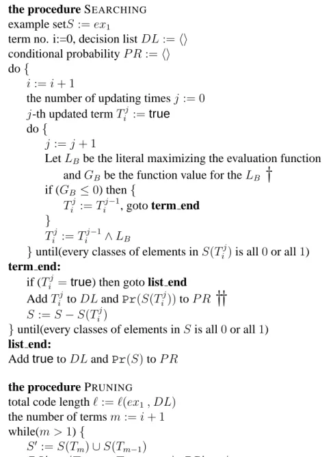
example set, ex

, and then the function is acquired from this new set.

To acquire f

(p

), it is required examples that are pairs of an observed value vector and a target value, i.e. A

(p

) and in(p

, π

) (a common format for the technique of learning from examples). We therefore transform a given example set EX into a set of examples in this form. Each example is generated from an object pair in an object set from the original example set. Thus, the number of elements in the transformed example set is the sum of the object pairs in the training example set, i.e. #ex

= P

I=1

#P

. We denote a transformed example by (A

(p

) , c), where the objects and object pairs are assumed to come from the same example (O

, π

). And where the class c takes the value in(p

, π

), so the c becomes 0 or 1. The value vector A

(p

) is calculated by combining the three attributes A(o

), A(o

), and A(p

). Our combination procedure is defined so as to be invariant under the ordering of indices, so that the value of the combined attribute A

(p

) is always equal to A

(p

). To produce such combined vectors, we copy all the values of A(p

) into the top of the combined vector. Additional elements are then concatenated to this combined vector by considering, one by one, the elements of the original vectors A(o

) and A(o

). The s-th elements of these original vectors, a

(o

) and a

(o

), are merged and added to the combined vector according to the following rules:

• If these two s-th elements take continuous values, the smaller value is added as an

element of the combined vector, and the larger value is added as the subsequent

element. That is, if the smaller value is added to the combined value as the t-th

element, the larger value would be added as the (t + 1)-th element.

5.1. ACQUISITION OF THE FUNCTION: F

(P ) 35

• If these two s-th elements take discrete values, the values are merged into one and added into the combined vector. If the number of possible values for the original attribute is d, the merged attribute can take one of a possible d(d + 1)/2 values. For example, if the possible values are “yes” and “no”, the merged value can take one of the values “yes–yes”, “yes–no”, or “no–no”.

As an example, consider the value vector A(p

) with two elements, the first discrete and the second continuous, and the vectors A(o

) and A(o

) both of which are with two elements, the first continuous and the second discrete. Given the attribute values A(p

) = (yes , 100), A(o

) = (50 , yes), and A(o

) = (10 , no), the combined attribute A

(p

) would be (yes , 100 , 10 , 50 , yes-no).

5.1.1 Our Algorithm to Estimate The Function: f

(p)

We next describe the algorithm to estimate the function f

(p) from the transformed ex- ample set, ex

. The example set can be simply represented by a form of {(A

, c

) , (A

, c

) , . . ., (A

, c

)}, where c

= {0 , 1} is a value of the function in(p , π

), and A

= (a

, a

, . . . , a

) denotes the combined attribute value vector A

(p). This algorithm finds the conditional probability function, Pr[c

=1|A

] for an unseen vector A

.

Before turning to the acquisition method of the probability function, we first present

the decision lists [31] used for representing the function. Let T be a term that is the

conjunction of literals L. The literal L is a logical function that can take the binary values

true or false when an attribute values a is given, as follows: