nucleon and 3,4 He elastic scattering

九州大学学術情報リポジトリ

Kyushu University Institutional Repository

核子および3,4He弾性散乱への微視的アプローチ

豊川, 将一

https://doi.org/10.15017/1806809

出版情報：Kyushu University, 2016, 博士（理学）, 課程博士 バージョン：

権利関係：Fulltext available.

Microscopic approach to

nucleon and ^3,4 He elastic scattering

Masakazu Toyokawa

Theoretical Nuclear Physics, Department of Physics

Graduate School of Science, Kyushu University

744, Motooka, Nishi-ku, Fukuoka 819-0395, Japan

Abstract

Properties of stable and unstable nuclei are clarified through nuclear reactions. It is im- portant to describe the nuclear reactions microscopically from the degrees-of-freedom of nucleons in order to analyze the nuclear reactions accurately and systematically. In this sense, microscopic understanding of nucleon-nucleus and nucleus-nucleus optical potential is the first goal on this line. In fact, the optical potentials are necessary to describe not only elastic scattering but also inelastic scattering, breakup and transfer reactions as key inputs in calculations of the distorted-wave Born approximation and the continuum discretized coupled-channels method (CDCC).

The main purpose of this thesis is to construct a microscopic framework of elastic scattering for nucleon and

He based on the multiple scattering theory. For this purpose, we construct reliable folding models. In the folding models, the g-matrix effective interaction is usually used as the effective nucleon-nucleon interaction by using the local-density approximation.

First we consider nucleon elastic scattering. For the scattering, the Melbourne group analyzed the scattering with the nonlocal version of the Melbourne g-matrix folding model. However, the nonlocal potential is not suitable for many applications.

We then localize the potential with the Brieva-Rook localization method and analyze nucleon elastic scattering in a wide range of incident energies with success in repro- ducing the experimental data. In addition, we verify that the chiral g matrix also reproduces the experimental data. This indicates that nuclear-force dependence is not essential.

Second we consider

He elastic scattering. For the scattering, we propose a new microscopic model. That is the double-folding (DF) model with the target-density approximation (TDA). In the DF-TDA model, the nuclear-matter density ρ in the g matrix is replaced by the local density of target nucleus. Projectile-excitation effects are not included in the model, but

He and

He are expected to be hardly excited in the reaction processes. In fact, we show that the projectile-excitation effects are small on

He elastic scattering by performing CDCC calculations. This verifies the validity of the DF-TDA model for

He elastic scattering, because

He is less fragile than

3

He. We also propose the double-single-folding (DSF) model as a simple and practical version of the DF-TDA model. In the DSF model, the optical potential is calculated from the local nucleon-nucleus folding potential and the projectile density. The DSF model well emulates the DF-TDA model at the angles where the experimental data

i

ii

are available. Both the models reproduce the experimental data with no adjustable

parameter.

Contents

Abstract i

1 Introduction 1

1.1 Nuclear reactions . . . . 1

1.2 Microscopic description of nuclear reaction . . . . 5

1.3 Purposes . . . . 8

2 Nucleon elastic scattering 11 2.1 Introduction . . . . 11

2.2 Theoretical framework . . . . 11

2.2.1 Microscopic description for nucleon-nucleus scattering . . . . 11

2.2.2 Single-folding model . . . . 14

2.2.3 Brieva-Rook localization . . . . 15

2.2.4 Spin-orbit potential . . . . 17

2.2.5 Melbourne g matrix . . . . 18

2.2.6 Nuclear-density calculation . . . . 19

2.3 Results . . . . 21

2.4 Short summary . . . . 28

3

He elastic scattering 29 3.1 Introduction . . . . 29

3.2 Theoretical framework . . . . 29

3.2.1 Microscopic description for nucleus-nucleus scattering . . . . 29

3.2.2 Double-folding model . . . . 31

3.2.3 Microscopic description for

He scattering . . . . 33

3.2.4 Basic framework of CDCC method . . . . 35

3.2.5 Spin-orbit potential for

He scattering . . . . 37

3.3 Results . . . . 39

3.3.1

He scattering . . . . 39

3.3.2

He scattering . . . . 43

3.4 Short summary . . . . 47

4 Summary 53

iii

iv CONTENTS

Acknowledgments 55

List of Figures

1.1 Nuclear chart . . . . 1

1.2 Schematic figure of the reaction processes . . . . 2

1.3 CDCC results for d elastic scattering on

Ni target at E

/A

= 40 MeV 3 1.4 Schematic figure of the inputs for CDCC calculation . . . . 3

1.5 Global optical potential analysis of proton elastic scattering . . . . 4

1.6 Analysis of proton elastic scattering with the Melbourne g-matrix fold- ing model . . . . 7

2.1 Coordinates for nucleon-nucleus scattering . . . . 12

2.2 dσ/dΩ and A

for proton elastic scattering on

C,

Ca,

Ni, and

Pb targets at E

= 65 MeV . . . . 22

2.3 σ

for proton elastic scattering on various kinds of targets at 47 ≤ E

≤ 65 MeV . . . . 22

2.4 dσ/dΩ and A

for proton elastic scattering on

C target at E

= 30– 200 MeV . . . . 24

2.5 dσ/dΩ and A

for proton elastic scattering on

Ca target at E

= 30– 201 MeV . . . . 24

2.6 dσ/dΩ and A

for proton elastic scattering on

Ni target at E

= 30– 192 MeV . . . . 25

2.7 dσ/dΩ and A

for proton elastic scattering on

Pb target at E

= 30– 200 MeV . . . . 25

2.8 dσ/dΩ for neutron elastic scattering on

C target at E

= 65–185 MeV 26 2.9 dσ/dΩ for neutron elastic scattering on

Ca target at E

= 65–185 MeV 27 2.10 dσ/dΩ for neutron elastic scattering on

Pb target at E

= 65–185 MeV . . . . 27

2.11 dσ/dΩ and A

for proton elastic scattering on

Pb target at E

= 30– 200 MeV based on chiral two-nucleon force . . . . 28

3.1 Coordinates for nucleus-nucleus scattering . . . . 30

3.2 Schematic figure of CDCC discretization . . . . 36

3.3 Coordinates for DSF spin-orbit potential . . . . 38

3.4 dσ/dΩ for

He elastic scattering on

Ni target at E

/A

= 40–148 MeV 40 3.5 σ

for

He elastic scattering on

Ni target . . . . 41

v

vi LIST OF FIGURES 3.6 Microscopic optical potentials for

He elastic scattering on

Ni target

at E

/A

= 40 and 148 MeV . . . . 42 3.7 Projectile-breakup and spin-orbit effects on dσ/dΩ for

He+

Ni elastic

scattering . . . . 43

3.8 Projectile-breakup effects on σ

for

He+

Ni elastic scattering . . . . . 44

3.9 dσ/dΩ for

He elastic scattering on

C target at E

/A

= 24–150 MeV 44

3.10 σ

for

He elastic scattering on

C target at E

/A

= 24–150 MeV . . 45

3.11 dσ/dΩ for

He elastic scattering on

Ca target at E

/A

= 43–72 MeV 45

3.12 σ

for

He elastic scattering on

Ca target at E

/A

= 32–72 MeV . . 46

3.13 dσ/dΩ for

He elastic scattering on

Pb target E

/A

= 43–150 MeV 46

3.14 σ

for

He elastic scattering on

Pb target E

/A

= 32–150 MeV . . 47

3.15 dσ/dΩ for

He elastic scattering on

Ni target at E

/A

= 21–175 MeV 48

3.16 σ

for

He elastic scattering on

Ni target at E

/A

= 20–175 MeV . 48

3.17 dσ/dΩ for

He elastic scattering on

C target at E

/A

= 26–98 MeV 49

3.18 σ

for

He elastic scattering on

C target at E

/A

= 14–98 MeV . . 49

3.19 dσ/dΩ for

He elastic scattering on

Ca target at E

/A

= 20–60 MeV 50

3.20 dσ/dΩ for

He elastic scattering on

Pb target at E

/A

= 26–175 MeV 50

3.21 σ

for

He elastic scattering on

Pb target at E

/A

= 26–175 MeV . 51

Chapter 1 Introduction

1.1 Nuclear reactions

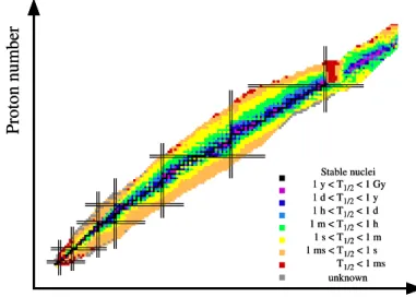
Atomic nucleus is a quantum many-body system composed of finite number of nu- cleons. Nucleon is classified into proton having a positive charge and neutron having no charge. Nuclei are characterized by the numbers of protons and neutrons, N and Z. Figure 1.1 is the nuclear chart, in which observed nuclei are plotted by N as the horizontal axis and Z as the vertical axis. The observed nuclei are classified by their lifetimes and shown by different colors in Fig. 1.1; the symbols painted in black denote stable nuclei with long lifetimes, and the symbols painted in other colors are unstable nuclei with short lifetimes that easily decay into other nuclide. There are about 300 kinds of stable nuclei in nature, and more than 3000 kinds of unstable nuclei have been measured experimentally. Most of the stable nuclei have characteristic properties such

Neutron number

Proton number

Stable nuclei 1 y < T_1/2 < 1 Gy 1 d < T_1/2 < 1 y 1 h < T_1/2 < 1 d 1 m < T_1/2 < 1 h 1 s < T_1/2 < 1 m 1 ms < T_1/2 < 1 s

T_1/2 < 1 ms unknown

Neutron number

Proton number

Stable nuclei 1 y < T_1/2 < 1 Gy 1 d < T_1/2 < 1 y 1 h < T_1/2 < 1 d 1 m < T_1/2 < 1 h 1 s < T_1/2 < 1 m 1 ms < T_1/2 < 1 s

T_1/2 < 1 ms unknown

Figure 1.1: Nuclear chart in which nuclei are plotted by the neutron number N as the horizontal axis and the proton number Z as the vertical axis. The colored symbols classify nuclei with the value of lifetime. The data are taken from Ref. [1].

1

2 Chap. 1 Introduction

Figure 1.2: Schematic figure of the reaction processes.

as the saturation property and the magicity. The saturation property means that the matter density of nucleus is saturated into some value at the center of nucleus. This property leads to the fact that the radii R of stable nuclei are well estimated by the mass number A of nuclei as R ∝ A

. Some nuclei with particular proton and neutron numbers, Z = 2, 8, 20, 28, 82, 126 and N = 2, 8, 20, 28, 82, 126, become more stable than the others. These numbers are called magic numbers, and this property is called the magicity.

The properties of nuclei have been studied mainly through nuclear reactions. Nu- clear reactions are the general term for collisions between nuclei, and are composed of many processes, as shown in Fig. 1.2. One can divide the nuclear reactions into elas- tic scattering as a basic process and non-elastic processes as higher-order processes.

Elastic scattering is the most fundamental process of nuclear reactions. We can un- derstand the elastic scattering by the optical model. In the optical model, elastic scattering is described by the one-body optical potential U that is composed of the real and imaginary parts: U = V + iW . The imaginary part W means the outflow of the incident flux to non-elastic channels. In general, the optical potential includes back-coupling effects from non-elastic channels implicitly.

The optical potentials are necessary to describe not only elastic scattering but also higher-order processes such as inelastic scattering, breakup and transfer reactions, and so on. In fact, the optical potentials are key inputs in the higher-order calculations based on the coupled-channel (CC) method, the distorted-wave Born approximation (DWBA) and the continuum discretized coupled-channel method (CDCC) [3, 4, 5].

CDCC is the method for describing excitation and breakup processes in scattering

of two- or three-body projectiles. The optical potentials between each constituent of

the projectile and the target nucleus are necessary for CDCC calculations. Figure

1.3 shows the results of CDCC calculations for deuteron (d) elastic scattering on

Ni

target at the incident energy E

= 80 MeV [2]. The difference between the solid and

dashed lines means d-breakup effects on the scattering. We can see from Fig. 1.3 that

d elastic scattering is well described with CDCC by including the d-breakup effects,

1.1 Nuclear reactions 3

Figure 1.3: Angular distribution of differential cross section dσ/dΩ divided by the Rutherford cross section (dσ/dΩ)

for d elastic scattering on

Ni target at E

/A

= 40 MeV. The solid line represents the results of CDCC calculation that includes d- breakup effects, while the dashed line denotes the results of one-channel calculation without the effects. The figure is taken from Ref. [2].

Figure 1.4: Schematic figure of the inputs for CDCC calculation shown in Fig. 1.3.

U

(U

) stands for the optical potential between proton (neutron) in deuteron

and

Ni target.

4 Chap. 1 Introduction since d is a weakly-bound nucleus and easily broken up into proton and neutron in the scattering. In the CDCC calculation, the optical potentials between each nucleon in d and

Ni target are used, as shown in Fig. 1.4.

So far the optical potentials were determined phenomenologically for stable nuclei from abundant experimental data, because the experiments of the collisions among stable nuclei are relatively easy in comparison with the experiments of radioactive isotope (RI) beams. In fact, several global optical potentials [6, 7, 8, 9] were proposed phenomenologically and used for the analyses of nuclear reactions between stable nu- clei. The global optical potentials were constructed by reproducing the experimental data in a wide range of incident energies and target mass numbers. Figure 1.5 shows the results of the global optical potential provided by A. J. Koning and J. P. Delaroche for proton elastic scattering on

Ni target at E

= 10–200 MeV [6]. In the Koning- Delaroche global optical potential, the potentials are described by the Woods-Saxon form. The parameters are provided as a function of N , Z , and E

. For proton scatter- ing from stable nuclei, the optical potentials are well determined phenomenologically, as shown in Fig. 1.5.

Figure 1.5: Angular destribution of differential cross sections dσ/dΩ divided by the Rutherford cross section (dσ/dΩ)

for proton elastic scattering on

Ni target at E

= 10–200 MeV. The dashed lines are the results of global optical potential, while the solid lines represent the results of fine-tuned potentials for each target nucleus.

The figure is taken from Ref. [6].

Recently, the study on nuclear physics has been moved from stable nuclei to un-

stable nuclei in virtue of the progress of experimental technique associated with RI

beams. It is well known that some unstable nuclei have exotic properties represented

by the halo structure. The halo structure is realized in a weakly-bound system com-

posed of a core nucleus and one or two neutrons. Halo nucleus has a radius much

larger than the stable nucleus with the same mass number. In principle, properties

1.2 Microscopic description of nuclear reaction 5 of unstable nuclei can be studied through nuclear reactions. In practice, it is quite difficult to construct accurate optical potentials for scattering between stable and un- stable nuclei phenomenologically because of limited observables for the scattering. In the experiments based on the inverse kinematics, unstable nuclei are employed as pro- jectiles, but the intensity of RI beams is much weak. The global optical potentials determined from the scattering between stable nuclei cannot be applied for the scat- tering of unstable nuclei, because the potentials do not emulate exotic properties of unstable nuclei. In addition, for the scattering of both stable and unstable nuclei, it is generally difficult to determine nuclear structure such as nuclear density ρ from ob- servables such as differential cross section dσ/dΩ quantitatively, without microscopic analyses of nuclear reactions. Therefore we should derive the optical potential not phenomenologically but microscopically.

1.2 Microscopic description of nuclear reaction

Nucleus is a quantum many-body system composed of finite number of nucleons in- teracting with nuclear force ˆ v. In principle, nuclear reactions can be described micro- scopically by the many-body Schr¨ odinger equation with the bare nuclear force.

So far, many kinds of phenomenological nuclear forces were constructed on the basis of the meson-exchange model proposed by H. Yukawa [10]. Recently, new types of nuclear forces have been constructed theoretically with Lattice-QCD [11] and chiral effective field theory (Ch-EFT) [12, 13]. In particular, the nuclear force based on Ch- EFT is extensively used for analyses of nuclear structure [14], nuclear matter [15, 16], and nuclear reaction [17, 18].

Microscopic description of nuclear reactions is one of important subjects in nuclear physics, but it is quite difficult to solve the many-body Schr¨ odinger equation exactly.

Therefore, we need the microscopic framework that allows us to solve the equation as accurately as possible.

Nucleon-nucleus elastic scattering

Microscopic description of elastic scattering comes down to constructing the optical potential based on nuclear force. Namely the optical potential is an essential building block in the microscopic framework of nuclear reactions. The optical model is derived microscopically by the Feshbach theory [19, 20]. For simplicity, we first consider nucleon elastic scattering from target nucleus (T). In the Feshbach theory, the optical potential is written by

U ˆ = ⟨ Φ

| P ˆ V ˆ P ˆ | Φ

⟩ + ⟨ Φ

| P ˆ V ˆ Q ˆ 1

E − Q ˆ H ˆ Q ˆ + iε

Q ˆ V ˆ P ˆ | Φ

⟩ (1.1) with

V ˆ = ∑

j

ˆ

v

, (1.2)

6 Chap. 1 Introduction where Φ

is the ground-state wave-function of T, and ˆ H represents the Hamiltonian of the total system. The operator ˆ P = | Φ

⟩⟨ Φ

| is the projection operator onto the ground-state of T, and the space spanned by Φ

is called P -space. Meanwhile, the operator ˆ Q = 1 − P ˆ is the projection operator onto all the excited states of T, and the space spanned by all the excited states is called Q-space. The relationship between the optical potential and Φ

is clearly seen in Eq. (1.1). This allows us to connect observables with nuclear structure. Since the nuclear force ˆ v

is real, the first term on the right-hand side of Eq. (1.1) becomes also real and hence does not include any back-coupling effect from Q-space to P -space. The second term on the right-hand side of Eq. (1.1) represents transition processes from P -space to P -space through Q-space.

All the back-coupling effects from Q-space are included in the second term on the right- hand side of Eq. (1.1) and the term thus makes the optical potential complex. Since the second term on the right-hand side of Eq. (1.1) contains the internal Hamiltonian of T that is a many-body operator, the microscopic optical potential becomes complex as a consequence of the many-body structure and the antisymmetrization of T.

In principle, we can obtain the optical potential from the nuclear force ˆ v by using Eq. (1.1). In practice, deriving the second term on the right-hand side of Eq. (1.1) is nothing but solving the many-body Schr¨ odinger equation. We introduce the effective interaction ˆ τ

instead of solving the second term on the right-hand side of Eq. (1.1).

The effective interaction ˆ τ

is constructed from the bare nuclear force ˆ v

by using the multiple scattering theory [21, 22, 23]. The effective interaction ˆ τ

includes the effects of the second term considerably, since ˆ τ

is the many-body operator including the excitations of T. We may then consider the following approximation is good:

U ˆ ≃ ⟨ Φ

| ∑

j

ˆ

τ

| Φ

⟩ . (1.3)

However, the effective interaction ˆ τ

is difficult to obtain exactly in the multiple scattering theory, since ˆ τ

is a many-body operator. As the standard approach, the g-matrix effective interaction ˆ g

is used instead of ˆ τ

by using the local-density ap- proximation. The g matrix is defined as the effective nucleon-nucleon interaction in symmetric nuclear matter, and depends on the density of nuclear matter ρ; ˆ g

= ˆ g

(ρ).

In the local density approximation, the density ρ in ˆ g

(ρ) is evaluated by the local density ρ

of T as ˆ g

(ρ) = ˆ g

(ρ

). Eventually, the optical potential is approximately described as

U ˆ ≃ ⟨ Φ

| ∑

j

ˆ

g

(ρ

) | Φ

⟩ . (1.4) This procedure is called the g-matrix folding model, and the right-hand side of Eq.

(1.4) is the g-matrix folding potential. The folding model includes not only the direct

processes but also the knock-on exchange processes between interacting two nucleons

as a part of the antisymmetrization of the total system. The later processes make the

folding potential nonlocal.

1.2 Microscopic description of nuclear reaction 7 Figure 1.6 shows the angular distribution of the differential cross sections dσ/dΩ for proton elastic scattering on various targets at E

= 65 MeV. The solid lines denote the results of the g-matrix folding model with the Melbourne g matrix [24], in which the folding potential is nonlocal. The Melbourne g-matrix folding model succeeded in reproducing the experimental data. However, the nonlocal potential makes numerical calculations more complicated not only for elastic scattering but also for higher-order processes such as inelastic scattering, breakup and transfer reactions. When we apply the microscopic optical potential to the higher-order processes, the nonlocal potential is quite inconvenient in the calculations. The nonlocality of the folding potential can be localized by the Brieva-Rook method [25, 26, 27]. The validity of the approximation is confirmed in Refs. [28, 29]. In this thesis, we will verify the reliability of the local version of the Melbourne g -matrix folding model. In the calculations of the higher- order processes, we can then use the local version of the Melbourne g-matrix folding potential as a reliable potential.

Figure 1.6: Angular distribution of differential cross sections dσ/dΩ for proton elastic scattering on various targets at E

= 65 MeV. The solid lines represent the results of the Melbourne g-matrix folding model that performed by the Melbourne group. The figure is taken from Ref. [24].

Nucleus-nucleus elastic scattering

Nucleus-nucleus elastic scattering can be described with the effective interaction ˆ τ

by extending the folding model as

U ˆ

= ⟨ Φ

Φ

| ∑

ij

ˆ

τ

| Φ

Φ

⟩ . (1.5)

8 Chap. 1 Introduction Here Φ

is the ground-state wave-function of projectile (P). This procedure is called double-folding (DF) model. However, the nucleon-nucleon multiple scattering series in nucleus-nucleus scattering is much complicated than that in nucleon-nucleus scat- tering. In fact, we have to consider excitations of not only target nucleus but also projectile nucleus. When we replace the effective interaction ˆ τ

by the g-matrix, we need to derive the g matrix by taking account of double fermi-sphere. The g matrix ˆ g

for nucleus-nucleus scattering depends on the densities, ρ

and ρ

, of P and T; ˆ g

= ˆ g

(ρ

, ρ

). However, it is not easy to formulate the g ma- trix itself for the double fermi-sphere. For this reason, the g matrix in the single fermi-sphere is used commonly by assuming the frozen-density approximation (FDA):

ˆ

g

(ρ

, ρ

) = ˆ g

(ρ

+ ρ

). There is an inconsistency between the framework of the effective interaction in nuclear matter and the DF model used in nuclear reactions.

Thus, there is no unified framework that describes nucleon-nucleus and nucleus-nucleus scattering simultaneously. As mentioned above, nucleon-nucleus scattering is easier than nucleus-nucleus scattering from the viewpoint of the multiple scattering theory.

We then start with the multiple scattering theory for nucleon-nucleus scattering, and extend the framework to

He- and

He-nucleus scattering that are not fragile and hence close to nucleon.

1.3 Purposes

The main purpose of this thesis is to construct a microscopic framework of elastic scattering of nucleon and

He that are not or less fragile. For this purpose, we start with the multiple scattering theory [21, 22, 23] and construct reliable folding models.

In the folding models, the g-matrix effective interaction is used as the nucleon-nucleon effective interaction by using the local-density approximation, as usual.

In Chap. 2, we consider elastic scattering of polarized nucleon on various target nu- clei. For the scattering, the Melbourne group has already analyzed the scattering with the Melbourne g-matrix folding model in which the folding potential is “nonlocal”[24], and has succeeded in reproducing the experimental data for the scattering. However, the nonlocal folding potential is not useful in applications for inelastic scattering, transfer and breakup reactions. We first propose the local version of the Melbourne g-matrix folding model and apply the model to nucleon elastic scattering on

C,

Ca,

58

Ni, and

Pb targets in a wide range of incident energies E

= 30–200 MeV. We show that the Brieva-Rook localization [25, 26, 27] taken is good. We also apply an- other g matrix constructed in Refs. [16, 18] from the chiral two-nucleon force [30] to proton elastic scattering on

Pb target at E

= 30–200 MeV in order to investigate nuclear-force (ˆ v ) dependence. This chapter is based on the following two papers:

• “Mass-number and isotope dependence of local microscopic optical potentials for polarized proton scattering”

M. Toyokawa, K. Minomo, and M. Yahiro,

1.3 Purposes 9 Phys. Rev. C 88, 054602 (2013).

• “Effects of chiral three-nucleon forces on proton- and

He-nucleus scattering in a wide range of incident energies”

M. Toyokawa, M. Yahiro, T. Matsumoto, and M. Kohno, to be submitted to Physical Review C.

In Chap. 3, we consider elastic scattering of

He and

He on various target nuclei in a wide range of incident energies. For the scattering, we propose a new microscopic model by using the multiple scattering theory [21, 22, 23] and apply the model to the scattering. The microscopic double-folding (DF) model proposed so far includes implicitly projectile-excitation effects on the scattering as well as target-excitation ef- fects. However, the projectile-excitation effects are considered to be small on the

He and

He elastic scattering, because these projectiles are not fragile and hardly excited.

Taking account of this property, we propose the microscopic model that projectile- excitation effects are not included. We then evaluate projectile-excitation effects on

3

He elastic scattering by CDCC calculations. From this analysis, we show that the effects are small on the scattering and confirm the validity of new microscopic model.

In this thesis, the model is referred to as DF model with the target-density approxi- mation (TDA). The DF-TDA model well reproduces the experimental data in a wide range of incident energies. We also propose the double-single-folding (DSF) model as a practical version of the DF-TDA model. In the DSF model, the optical potential is calculated from the local nucleon-nucleus folding potential and the projectile density.

The DSF and DF-TDA models are different only for the knock-on exchange processes.

Comparing the two models, we show that the DSF model simulates the DF-TDA model with good accuracy at the angles where the experimental data are available.

This chapter is based on the following two papers:

• “Microscopic optical potentials for

He scattering”

K. Egashira, K. Minomo, M. Toyokawa, T. Matsumoto, and M. Yahiro, Phys. Rev. C 89, 064611 (2014).

• “Microscopic approach to

He scattering”

M. Toyokawa, T. Matsumoto, K. Minomo, and M. Yahiro,

Phys. Rev. C 91, 064610 (2015).

Chapter 2

Nucleon elastic scattering

2.1 Introduction

In this chapter, we make systematic analyses of nucleon-nucleus elastic scattering on various targets in a wide range of incident energies E

= 30–200 MeV with a local version of the g-matrix folding model. Nucleon-nucleus elastic scattering can be de- scribed microscopically by the folding model based on the multiple scattering theory [21, 22, 23]. The folding model allows us to construct the nucleon-nucleus optical potential from the nucleon-nucleon effective interaction and the density of target nu- cleus. In the folding model, the g-matrix effective interaction is commonly used as the nucleon-nucleon effective interaction by using the local-density approximation. The knock-on exchange processes, originating in the antisymmetrization of nucleons, make the optical potential nonlocal. The nonlocal version of the g-matrix folding model proposed by Melbourne group is successful in reproducing the experimental data for nucleon elastic scattering on various targets [24]. However the nonlocal optical poten- tial is quite inconvenient in many applications. Hence we confirm that the nonlocality can be localized by the Brieva-Rook method [25, 26, 27] with good accuracy, and show that the local version of the Melbourne g matrix is also successful in reproducing the experimental data. Finally, we show that nuclear-force (ˆ v ) dependence is small by per- forming the same calculation with the g matrix constructed from chiral two-nucleon force for proton elastic scattering on

Pb target.

2.2 Theoretical framework

2.2.1 Microscopic description for nucleon-nucleus scattering

Microscopic description of nucleon scattering on a target (T) should be governed by the many-body Schr¨ odinger equation

(

K ˆ

+ ˆ h

+ ∑

j∈T

ˆ v

− E

)

| Ψ

⟩ = 0 (2.1)

11

12 Chap. 2 Nucleon elastic scattering for the total wave-function Ψ

with the outgoing boundary condition. Here ˆ v

represents the bare nucleon-nucleon interaction between the incident nucleon labeled by 0 and the j-th nucleon in the target nucleus. Figure 2.1 shows the definition of coordinates needed to describe nucleon-nucleus scattering. The coordinate R means the location of the incident nucleon 0 from the center-of-mass (c.m.) of T. The operator K ˆ

represents the kinetic energy associated with the relative coordinate R. The operator ˆ h

corresponds to the internal Hamiltonian of T. The constant E is the total energy of the present system and is related to the ground-state energy ε

of T and the relative energy E

between the incident nucleon 0 and T in the c.m. frame as

E = E

+ ε

, (2.2)

where note that ε

is negative. The relative energy E

is written as E

= m

m

+ m

E

(2.3)

with the incident energy E

of nucleon 0 in the laboratory frame and the masses, m

and m

, of nucleon 0 and target nucleus T.

Figure 2.1: Definition of coordinates for nucleon-nucleus scattering. R and r represent the coordinates of the incident nucleon and the internal nucleon in target from the center-of-mass of target. s denotes the relative coordinate among interacting two nucleons.

The multiple scattering theory [21, 22, 23] allows us to derive the many-body Schr¨ odinger equation

(

K ˆ

+ ˆ h

+ A

− 1 A

∑

j∈T

ˆ τ

− E

)

| Ψ

⟩ = 0 (2.4)

from the original equation (2.1). When the mass number A

of T is much larger than 1, the factor

T

can be approximated into 1. In Eq. (2.4), a collision between the

2.2 Theoretical framework 13 incident nucleon 0 and the j-th nucleon in T is described by the effective nucleon- nucleon interaction τ ˆ

instead of the bare nucleon-nucleon interaction ˆ v

. In the multiple scattering theory, ˆ τ

is obtained from ˆ v

as

ˆ

τ

= ˆ v

+ ˆ v

G ˆ

τ ˆ

, (2.5) with the propagator

G ˆ

=

P ˆ

E − ( ˆ K

+ ˆ h

) + iϵ . (2.6) The operator ˆ P

has been introduced to require that the ground-state wave-function Φ

of T should be antisymmetrized. When Eq. (2.4) is derived from Eq. (2.5), we have neglected the antisymmetrization between the incident nucleon 0 and the nucleons of T. However, it is shown in Refs. [31, 32] that the antisymmetrization effects are well described by direct and knock-on exchange processes between interacting two nucleons for higher incident energies E

≳ 50 MeV. Thanks to the many-body operators ˆ P

and ˆ h

in Eq. (2.6), the effective nucleon-nucleon interaction ˆ τ

includes many-body effects, so-called medium effects. Solving Eq. (2.5) for finite nuclei is quite difficult, because it is nothing but solving the many-body problem. Therefore we need to obtain the effective interaction in an alternative way.

A candidate is to use the g matrix (ˆ g

) instead of ˆ τ

. The g matrix is defined as the effective nucleon-nucleon interaction in symmetric nuclear matter, and obtained by solving the Br¨ uckner-Bethe-Goldstone equation

ˆ

g = ˆ v + ˆ v Gˆ ˆ g , (2.7)

with the propagator

G ˆ =

Q ˆ

E − ( ˆ K + ˆ U ) + iϵ . (2.8)

Here ˆ Q is the Pauli blocking operator prohibiting transitions to the occupied levels below the Fermi surface. The operator ˆ U represents the single-particle potential

U ˆ = ∑

b

⟨ a, b | g ˆ | a, b ⟩ (2.9)

defined as a mean-field potential of nuclear matter, where the b denote the occupied states. Equations (2.7) and (2.9) show that ˆ g and ˆ U should be solved self-consistently.

This self-consistent procedure is called the Br¨ uckner-Hartree-Fock (BHF) method.

The resultant g matrix depends on the density ρ of nuclear matter: ˆ g

= ˆ g

(ρ).

When ˆ g

(ρ) is applied to nucleon-nucleus scattering, it is commonly assumed that

ρ = ρ

(r) , (2.10)

where ρ

(r) is the nuclear density of T at the location r of interacting two nucleons.

This is called the local-density approximation.

14 Chap. 2 Nucleon elastic scattering

2.2.2 Single-folding model

Introducing the projection operator ˆ P on the ground-state of T, we can describe the total wave-function Ψ

as

| Ψ

⟩ ≈ P ˆ | Ψ

⟩ = | Φ

χ

⟩ , (2.11) where Φ

is the ground-state wave-function of T, and χ

is the relative wave-function between the incident nucleon and the target nucleus. Hereafter, symbols µ and ν mean either proton or neutron. We then can reduce the many-body Schr¨ odinger equation (2.4) to the one-body Schr¨ odinger equation

[ K ˆ

+ ˆ U

− E

] | χ

⟩ = 0, (2.12)

by multiplying Φ

from the left-hand side of Eq. (2.4). Here U ˆ

= ⟨ Φ

| ∑

j

ˆ

g

(ρ) | Φ

⟩ (2.13)

is called “single-folding (SF) potential”and the one-body Schr¨ odinger equation (2.12) is “single-folding model”. In the single folding model, the inelastic channels are not treated explicitly, but the back-coupling effects on the elastic channel are included by using the g matrix.

Assuming the internal wave-function Φ

of T as the single slater-detarminant of single-particle wave-functions φ

, we can rewrite the folding potential (2.13) as

U ˆ

= ∑

α

⟨ φ

| ˆ g(ρ) | φ

⟩ (2.14)

where the label α means the single-particle state. Taking account of the knock-on exchange operator in ˆ g, one can rewrite the one-body Schr¨ odinger equation (2.12) in coordinate space as

[

− ℏ

2µ ∇

+ U

(R) − E

]

χ

(R) =

∫

drU

(r, R)χ

(r) (2.15) with the local direct term U

(R) and the nonlocal exchange term U

(r, R),

U

(R) = ∑

ν

∫

drρ

(r)g

(s, E

, ρ) , (2.16) U

(r, R) = ∑

ν

˜

ρ

(r, R)g

(s, E

, ρ) , (2.17) where ρ

and ˜ ρ

are the one-body and mixed target densities defined by

ρ

(r) = ∑

α

φ

(r)φ

(r) , (2.18)

˜

ρ

(r, R) = ∑

α

φ

(r)φ

(R), (2.19)

2.2 Theoretical framework 15 and the direct and knock-on exchange terms, g

and g

, are determinable from ˆ g as shown later in Sec. 2.2.5. In general, the one-body density is not spherical, so that U

(R) is composed of spherical and nonspherical components. However, the nonspherical component vanishes when the target spin is zero and is small even when it is nonzero [33]. Therefore we can assume that the one-body density and the direct- process part of the folding potential are spherical; ρ

(r) = ρ

(r) and U

(R) = U

(R). In this paper, as the standard choice, the nuclear-matter density ρ in g

and g

is assumed to agree with the target density at the midpoint of interacting two nucleons:

ρ = ρ

( | r − s/2 | ) . (2.20) Equation (2.15) allows us to describe nucleon elastic scattering on target nucleus with the microscopic optical potential constructed from the g-matrix effective inter- action and the one-body and mixed densities, ρ

(r) and ˜ ρ

(r, R), of target nucleus.

However the nonlocality in the knock-on exchange term U

(r, R) makes numeri- cal calculations much complicated, since it makes the Schr¨ odinger equation (2.15) an integro-differential equation. In addition, such a nonlocal potential is not useful for many applications of nuclear reactions such as inelastic scattering, breakup, and transfer reactions. Nevertheless, we will show that the nonlocal folding potential (2.17) can be localized accurately with the the Brieva-Rook method [25, 26, 27] for nucleon scattering.

2.2.3 Brieva-Rook localization

The Brieva-Rook localization is composed of the following three approximations:

1. local semi-classical approximation 2. local Fermi-gas approximation 3. isotropic approximation

We can simplify Eq. (2.15) with the trivially-equivalent local potential U

(R) defined by

U

(R) = 1 χ

(R)

∫

dr U

(r, R)χ

(r) . (2.21) By using the local semi-classical approximation, the relative wave-function χ

(r) is approximated into a product of χ

(R) and e

AT+1 AT s)

: χ

(r) = χ

(R + A

+ 1

A

s) ≃ χ

(R)e

AT+1 AT K(R)·s

, (2.22)

Here K (R) represents the local momentum at the coordinate R with the magnitude

determined from the local energy conservation, and the direction is assumed to be

16 Chap. 2 Nucleon elastic scattering paralleled to the flux of scattering wave:

ℏ K(R) =

√

2µ[E

− U

(R) + U

(R) − V

(R)δ

] , (2.23)

K(R) ˆ ∥ Re[χ

(R) ∇

χ

(R)] , (2.24)

where V

(R) is the Coulomb potential between the incident proton and T. Applying Eq. (2.22) to Eq. (2.21) leads to

U

(R) =

∫

dr U

(r, R)e

AT+1 AT K(R)·s

. (2.25)

The factor

T

can be well approximated into 1 when the mass number A

of T is large enough.

Next we approximate the nonlocal density (2.19) into a local one with the local Fermi-gas approximation:

˜

ρ

(r, R) = ∑

α

φ

(r)φ

(r − s)

≃ ∑

α

( φ

(r − s/2)e

)

φ

(r − s/2)e

= ρ

( | r − s/2 | )e

, (2.26) where k is the momentum of nucleon in T at the coordinate r − s/2. The plane wave e

is replaced by the averaged plane wave of free fermions, since the target density ρ

(r) is well described by Fermi gas in the vicinity of r [34]:

ρ

( | r − s/2 | )e

≃ ρ

( | r − s/2 | ) 3 4π(k

)

∫

≤k_F^(ν)

dk e

= ρ

( | r − s/2 | ) 3j

(k

s)

k

s , (2.27)

where k

is the Fermi momentum that is related to the density ρ

as k

( | r − s/2 | ) =

(

3π

ρ

( | r − s/2 | ) )

, (2.28)

and j

(x) is the spherical Bessel function of order 1.

Using the local semi-classical and the local Fermi-gas approximation, we can obtain the trivially-equivalent local potential as

U

(R) = ∑

ν

∫

dr ρ

( | r − s/2 | ) 3j

(k

s)

k

s g

(s, E

, ρ)e

AT+1 AT K(R)·s

. (2.29) However it is not easy to calculate, because the potential depends on the direction ˆ R of R. Usually the following isotropic approximation is taken for e

AT+1 AT K(R)·s

to avoid the complication [25, 26, 27]:

e

AT+1 AT K(R)·s

≃ 1

4π

∫

d R ˆ e

AT+1 AT K(R)·s

= j

(

T

K(R)s). (2.30)

2.2 Theoretical framework 17 Eventually, the local form of the nonlocal potential (2.17) is obtained as

U

(R) = ∑

ν

∫

dr ρ

( | r − s/2 | ) 3j

(k

s)

k

s g

(s, E

, ρ)j

(

T

K(R)s) . (2.31) As an advantage of the local version of the folding potential based on the Brieva-Rook method, we can say that only the one-body density ρ

(r) of the target nucleus is needed, that is, the single-particle wave-functions are not necessary. Therefore the local version of folding potential can be evaluated with both of phenomenological and microscopic one-body densities. We will mention how to obtain the one-body densities in Sec. 2.2.6.

2.2.4 Spin-orbit potential

So far, we discussed the central component of folding potential. However the potential between an incident nucleon and a target nucleus is composed of not only central component but also spin-orbit (LS) component. By using the folding model, we can construct the spin-orbit potential microscopically with the one-body density and the spin-orbit component of g-matrix effective interaction [35]:

U

(R) = − 1 4R

∑

ν

∫

dr R · s ρ

(r)g

(s, E

, ρ) (2.32) and

U

(R) = − π ∑

ν

∫ ds s

[ 2j

(K(R)s)

R ρ

(R, s) + j

(K(R)s)

2K δ

(R, s) ]

,(2.33)

where

δ

(R, s) = 1 2

∫

−1

dω g

(s, E

, ρ) x

×

 



3j

(k

s) k

s

d

dx ρ

(x)

√

R²+s²/4+Rsω

+sρ

(x) d

dx k

(x)

√

R²+s²/4+Rsω

× d dy

[ 3j

(y) y

]

y=k^(µ)_F s

}

, (2.34)

and

ρ

(R, s) = 1 2

∫

−1

dω ω g

(s, E

, ρ)

× 3j

(k

s)

k

s ρ

(x)

x=

√

R²+s²/4+Rsω

. (2.35)

18 Chap. 2 Nucleon elastic scattering

2.2.5 Melbourne g matrix

We have adopted the g matrix constructed by Melbourne group [24], so-called Mel- bourne g matrix, as the effective nucleon-nucleon interaction. Melbourne g matrix is obtained from the Bonn-B bare nucleon-nucleon interaction [36] by solving Br¨ uckner- Bethe-Goldstone equation (2.7). Since the solution to the Br¨ uckner-Bethe-Goldstone equation (2.7) is obtained nonlocally and numerically, the original g matrix is incon- venient for many applications. Therefore Melbourne group provided the local version of g matrix that is equivalent to the original g matrix for on-shell and near-on-shell matrix elements.

Melbourne g matrix is provided as g(s, E

, ρ) = ∑

i

∑

ST

ˆ

g

(s, E

, ρ) ˆ P

, (2.36) where the indices i represent the central (C), spin-orbit (LS), and tensor (T) compo- nents of the g matrix and the operator ˆ P

corresponds to the projection onto the total spin S and the total isospin T channel. The g

are written as

 

 

 

 

 

 



 

 

 

 

 

  ˆ

g

(s, E

, ρ) = ∑

j

a

(E

, ρ)f

(s)

ˆ

g

(s, E

, ρ) = ∑

j

b

(E

, ρ)f

(s)ℓ · (σ

+ σ

)

ˆ

g

(s, E

, ρ) = ∑

j

c

(E

, ρ)f

(s) ˆ S

(2.37)

with the Yukawa-type form factor

 

 

 

 

 

 

 

 

 

 

 



f

= exp[ − s/µ

] s

f

= exp[ − s/µ

] s

f

= s

exp[ − s/µ

] s

(2.38)

and ˆ S

is the tensor operator defined as

S ˆ

= 3(σ

· s)(σ

· s)

s

− σ

· σ

. (2.39)

The g matrix g

in Eqs. (2.16), (2.17), (2.32), and (2.33) can be described by the g

:

• For the direct-process part of proton-proton (neutron-neutron) interaction, g

= 1

4 (g

+ g

) , (2.40)

g

= g

. (2.41)

2.2 Theoretical framework 19

• For the direct-process part of proton-neutron (neutron-proton) interaction, g

= 1

8 (g

+ g

+ g

+ g

) , (2.42) g

= 1

2 (g

+ g

) . (2.43)

• For the knock-on exchange-process part of proton-proton (neutron-neutron) in- teraction,

g

= 1

4 ( − g

+ g

) , (2.44)

g

= g

. (2.45)

• For the knock-on exchange-process part of proton-neutron (neutron-proton) in- teraction,

g

= 1

8 (g

− g

− g

+ g

) , (2.46) g

= 1

2 ( − g

+ g

) . (2.47)

2.2.6 Nuclear-density calculation

We use two types of one-body densities in this study; one is the phenomenological density that is used for lighter nuclei A < 40 and the other is the Hartree-Fock (HF) density that is applied for heavier nuclei A ≥ 40. We will show how to obtain the phenomenological and HF densities in the following subsections, separately.

Hartree-Fock densities

For heavier nuclei, we have performed spherical HF calculations to obtain the one- body densities. The HF method is one of mean-field theories based on the independent particle model where each nucleon moves independently in a mean-field potential. The Schr¨ odinger equation for nucleus with the nucleon number A is written by

HΦ(x ˆ

, x

, · · · , x

) = EΦ(x

, x

, · · · x

) , (2.48) with the Hamiltonian

H ˆ =

∑

K ˆ

+

∑

∑

ˆ

v(x

, x

) . (2.49)

Here x

represents the coordinate, spin, and isospin of the i-th nucleon and Φ corre- sponds to the normalized A-body total wave-function. In the HF method, the total wave-function Φ(x

, x

, · · · , x

) is assumed as the single slater-detarminant of single- particle wave-functions φ

:

Φ(x

, x

, · · · , x

) = 1

√ A! det { φ

(x

) } , (2.50)