Fl ow
- of - f unds anal ys i s i n t he Br az i l i an
ec onom
y ( 2004 2014)
著者
Bur kow
s ki Er i ka, Ki m
J i young
権利
Copyr i ght s 日本貿易振興機構(ジェトロ)アジア
経済研究所 / I ns t i t ut e of D
evel opi ng
Ec onom
i es , J apan Ext er nal Tr ade O
r gani z at i on
( I D
E- J ETRO
) ht t p: / / w
w
w
. i de. go. j p
j our nal or
publ i c at i on t i t l e
I D
E D
i s c us s i on Paper
vol um
e
696
year
2018- 03
INSTITUTE OF DEVELOPING ECONOMIES
IDE Discussion Papers are preliminary materials circulated to stimulate discussions and critical comments
Keywords: flow-of-funds, financial crisis, Brazilian economy, asset–liability matrix, input-output JEL classification: C67, D53, G20, N26, O16
*Research Fellow, Global Value Chains Studies Group, Inter-disciplinary Studies Center, IDE
IDE DISCUSSION PAPER No. 696
Flow-of-Funds Analysis in the Brazilian
Economy (2004–2014)
Erika BURKOWSKI and Jiyoung KIM*
March 2018
Abstract
This paper applies the flow-of-funds (FOF) framework proposed by Tsujimura and Mizoshita (2004) to investigate the
structure of financial system in the Brazilian economy. The study presents the compilation process of the asset–liability
matrix (ALM) and then develops an ALM with six institutional sectors (households, non-financial firms, government,
the rest of world, financial firms and the Central Bank of Brazil) for the years 2004 to 2014. From the Brazilian ALM,
FOF indexes are calculated (the power of dispersion, the sensitivity of dispersion and the discrepancy of dispersion). For
selected years, the structural decomposition of change in the discrepancy index is calculated and an additional expansion
presents an ALM with four additional financial firms: three government-sponsored banks—Banco do Brasil, Caixa
Econômica Federal, and Banco Nacional de Desenvolvimento Econômico e Social —and one private bank—Itaú. The
role of each institutional sector in the Brazilian financial system is illustrated and the discrepancy of dispersion is
highlighted with a good indicator of economic problems showing that the origin of recessions in Brazilian economy was
The Institute of Developing Economies (IDE) is a semigovernmental,
nonpartisan, nonprofit research institute, founded in 1958. The Institute
merged with the Japan External Trade Organization (JETRO) on July 1, 1998.
The Institute conducts basic and comprehensive studies on economic and
related affairs in all developing countries and regions, including Asia, the
Middle East, Africa, Latin America, Oceania, and Eastern Europe.
The views expressed in this publication are those of the author(s). Publication does
not imply endorsement by the Institute of Developing Economies of any of the views
expressed within.
INSTITUTE OF DEVELOPING ECONOMIES (IDE), JETRO 3-2-2, WAKABA,MIHAMA-KU,CHIBA-SHI
CHIBA 261-8545, JAPAN
©2018 by Institute of Developing Economies, JETRO
Flow-of-Funds Analysis in the Brazilian Economy (2004–2014)
Erika BURKOWSKIa
Jiyoung KIMb
Abstract
This paper applies the flow-of-funds (FOF) framework proposed by Tsujimura and Mizoshita (2004) to investigate the structure of financial system in the Brazilian economy. The study presents the compilation process of the asset–liability matrix (ALM) and then develops an ALM with six institutional sectors (households, non-financial firms, government, the rest of world, financial firms and the Central Bank of Brazil) for the years 2004 to 2014. From the Brazilian ALM, FOF indexes are calculated (the power of dispersion, the sensitivity of dispersion and the discrepancy of dispersion). For selected years, the structural decomposition of change in the discrepancy index is calculated and an additional expansion presents an ALM with four additional financial firms: three government-sponsored banks—Banco do Brasil, Caixa Econômica Federal, and Banco Nacional de Desenvolvimento Econômico e Social —and one private bank—Itaú. The role of each institutional sector in the Brazilian financial system is illustrated and the discrepancy of dispersion is highlighted with a good indicator of economic problems showing that the origin of recessions in Brazilian economy was almost in the structure of the financial system.
Keywords: flow-of-funds, financial crisis, Brazilian economy, asset–liability matrix,
input-output
JEL classification: C67, D53, G20, N26, O16
Acknowledgements
The authors would like to thank Kazusuke Tsujimura and Masako Tsujimura for their
teachings about the theory, help in the treatment of data and support in the interpretation
of the results, which were extremely valuable contributions to the development of this
research.
a Departamento de Administração (VAD), Instituto de Ciências Humanase Sociais (ICHS), Universidade
Federal Fluminense (UFF), Brazil, e-mail: [email protected]
1. Introduction
Recent financial crises have shown that shocks in financial markets trigger
significant effects on the real side of the economy. The Brazilian economy suffered at
least two periods of recession in the last decade exemplified by a decrease in the total
Gross Domestic Product (GDP) in the years 2009 and 2014 (IBGE, 2017). It is not a
coincidence that in the prior year of each downturn, there was a high dispersion between
asset and liability discrepancy.
A particular feature of FOF analysis is its ability to show the linkage between
financial and objective economy because excess assets in the financial account represent
excess saving in the current account and excess liabilities in the financial account
represent excess investments in the current account. Thereafter, the sequence of the
accounts is not a one-way relation but consists of a loop. This loop explains the feedback
process between real and financial markets.
The FOF framework originates from Copland’s (1952) description of money flow.
From that four-entry system extracts an asset table and a liability table to derive an asset–
liability matrix (ALM). An ALM is a sector-by-sector square matrix, so input-output (IO)
methodology can be applied to extract information about a financial market. However,
one of the leading peculiarities of the FOF analysis is that two distinct sector-by-sector
ALMs can be derived from a single set of balance sheets. The first one describes the
propagation process of raising funds (the liability side) while the other one describes the
employment of funds (asset side). According to Tsujimura and Mizoshita (2004), when
there are discrepancies in the valuation of assets and liabilities, the magnitude of the
dispersion could be different in different systems. This magnitude will give us a clue to
the generation mechanism of financial bubbles.
Since developed countries have more detailed FOF accounts data compared with
developing countries, previous studies primarily used data from developed countries. For
examples, Zhang (1996) analyzed FOF of Japan and China. Nishiyama (2008) examined
a financial macroeconometric model using FOF of the United States. Kim (2008)
compared the financial systems of Japan and Korea, rearranging institutional sectors in
ALMs of the two countries. Moreover, Kim (2017) subdivided the non-financial private
corporations sector in a Korean ALM into chaebol (large-scale, family-run management
enterprises) and small- to medium-sized corporations. Some researchers have examined
transactions tables between multiple countries. Zhang (2009) built a model of the
global-FOF and estimated several multiple-equation models. However, case studies of
developing countries are scarce because of lack of data availability.
This study presents the details of the process of compiling an asset–liability matrix
(ALM) of the Brazilian economy from 2004 to 2014. The Brazilian ALM has six
institutional sectors (household, non-financial firms, the government, the rest of the world,
financial firms, and the central bank of Brazil) on both the liability side and the asset side
for the years 2004 to 2009 and 2009 to 2014. These two periods are defined because of
the availability of the data sources. For the period 2004–2009, the data came from
Brazilian Institute of Geography and Statistics (IBGE) and Central Bank of Brazil (BCB);
for the period 2009–2014, the data came from Organization for Economic Co-operation
Development (OECD) and BCB.
From Brazilian ALM, the Leontief inverse was calculated, and FOF indexes were
extracted. The power of dispersion and the sensitivity of dispersion indicate the role of
each institutional sector and its fluctuation in the financial market.
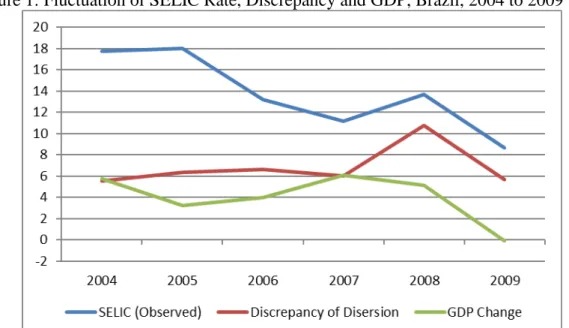
The discrepancy of dispersion indicates that 2009 and 2014, years of a high
decline in the GDP in the objective economy, were preceded by a high increase in the
difference of ALM total sum between the asset and liability side (2008 and 2013) and that
this great increase in discrepancy is concomitant of an increase in the interest rate
controlled by the monetary authority. Figure 1 plots the observed SELIC rate1, the
discrepancy of dispersion and the GDP fluctuation between 2004 and 2009.
The total sum of FOF in the years that presented the highest differences between
the total sum of ALM in the asset and liability side (2007 to 2008, and 2012 to 2013) was
decomposed to access the contribution from the financial structure and contribution from
the objective economy to total change in discrepancy. Moreover, an expanded ALM was
developed to include some important financial institutions to have a wide view of the
Brazilian financial system in 2009.
The novelty of the research is applying a FOF framework to the Brazilian
economy and corroborating that idea that FOF can be a useful tool to predict an economic
recession.
1 SELIC is the nominal interest rate of financing in the interbank market related to one day trade operations
Beyond this introduction, the paper presents the FOF analysis, including the
methodology to develop ALM, in calculating the indexes and the structural
decomposition analysis. Next, the methodology of empirical analysis, Brazilian data and
the results are presented.
Figure 1: Fluctuation of SELIC Rate, Discrepancy and GDP, Brazil, 2004 to 2009
Source: BCB (2017), IBGE (2017) and authors’ data
2. Flow-of-Funds
The FOF analysis was stimulated by the four entries system proposed by Copeland
(1952). Called the “system of money flow,” the four-entry system intended to presents
financial transactions using a table that records financial assets and liabilities, organized
with financial instruments (in the rows) held by each institutional sector (located in the
column). For each agent there are two columns: one for assets and other for liabilities.
With this model, it is possible to visualize the total assets, the total liabilities, and the
excess of assets and liabilities of institutional sectors and of a wide economy.
Since all financial transactions occur between at least two agents and for
management accountability each asset (liability) needs a corresponding liability (asset) in
the same amount, so financial transactions are registered in four accounts. Figure 2
represents Copland’s four-entry system, using financial assets and liabilities of Brazilian
Copeland’s four-entry system provides evidence solely for the financial assets and
liabilities. Since the balance sheet from business accounting method of any entity
represent all of the firm’s assets (financial and fixed) and liabilities (required and equity)
with a double entry, the excess of financial assets and excess of liabilities in the FOF
accounts represent respectively the excess of savings and the excess of investments in the
current account. In this way, FOF analysis can offer evidence of linkages between the
objective economy (production, income, gross fixed capital formation, and savings) and
the financial economy (employment of excess savings in financial asset and raising
liability to finance excess investment).
The FOF analysis evolves the application of the IO methodology to square
matrices, which represent the financial assets and liabilities transacted between the
institutional sectors (the ALM), which behaves as an IO matrix. In the ALM, however,
intermediate consumption refers to funds (financial assets and liabilities), rather than
goods and services. An IO matrix shows the demand (input) and the supply (output) of
goods, services and factors of production (intermediate production flow), while the ALM
shows the supply and demand of financial assets and liabilities (the “intermediate
financial flow”).
Although assets and liabilities represent counterparts of the same accounting entry,
changes in assets and changes in liabilities have distinct origins and effects. This is one
of the most important properties of FOF analysis (Tsujimura & Mizoshita, 2003b).
Table 1 represents the four-entry system proposed by Copeland (1952). It shows
the interrelation between the flow of financial assets and liabilities in the Brazilian
economy, the financial transactions of each agent and the transactions that occurred
among them. The vertical double entry ensures the internal consistency within an
institutional unit. For example, in the last row in Table 1 is observed that there is
consistency across entries (total assets + excess liability = total liability + excess assets
in each institutional sector).
Since each financial transaction involves at least two different agents, a creditor
and a debtor, the horizontal double entry assures the inter-consistency between
institutional units. In the last two columns in Table 1, the consistency is maintained
throughout the financial market (total assets = total liability and total excess = total assets
Table 1: Representation of Quadruple-Entry-System to Brazilian Economy, 2004 (R$ 1,000,000)
Source: Elaborated by authors from the Financial Balance Sheet of Brazil (2011) and Balance Sheet of Central Bank of Brazil (2004)
Institutional Sectors
Instruments ASSET LIABILITY ASSET LIABILITY ASSET LIABILITY ASSET LIABILITY ASSET LIABILITY ASSET LIABILITY ASSET LIABILITY
Cash and
Depósits 227,228 864,157 76,836 179,795 206,243 0 381,815 0 228,661 0 7,824 84,655 1,128,607 1,128,607
Bonds 942,146 340,188 384,828 13,644 100,487 112,963 40,952 1,228,089 46,959 0 281,205 101,693 1,796,578 1,796,578
Loans 819,069 264,712 22,869 228,167 110,422 461,218 461,639 518,530 9,514 193,655 244,521 1,752 1,668,034 1,668,034
Shares 814,491 1,336,120 0 0 1,220,302 1,765,791 219,413 0 411,859 0 588,038 152,192 3,254,102 3,254,102
Tecnichal
Insurance 1,481 316,383 0 3,831 4,932 0 142 0 312,953 0 706 0 320,214 320,214
Other
Deb./Credit 293,387 347,769 110 677 735,382 1,196,085 724,958 233,824 357,063 346,889 62,465 48,122 2,173,366 2,173,366
Difference 371,528 0 0 58,529 1,158,289 0 151,522 0 0 826,466 0 796,345 1,681,339 1,681,339
Total
2.1 E & R-Table
To develop the ALM and analyze the structure of financial flows, it is necessary
to first obtain the asset table and the liability table.
The asset table is composed by one matrix (the E-Matrix) with various assets
negotiated by various sectors and by additional vectors, which represent the excess of
liabilities in relation to the assets and the total by instrument and total by sector.
Where n is the number of financial instruments and m is the number of
institutional sectors, Equation 1 expresses the elements contained in the table of assets
(Tsujimura & Mizoshita, 2003a):
E = �
e11 e12 ⋯ e1m e21 e22 ⋯ e2m
⋮ ⋮ ⋱ ⋮
en1 en2 ⋯ enm �ε = �
ε1 ε2 ⋮ εm ��� = ⎣ ⎢ ⎢ ⎡s1E
s2E ⋮ snE⎦⎥
⎥ ⎤
z = �
z1 z2 ⋮ zm
� (E. 1)
where:
eij= amount of funds allocated to i-th financial instrument by the j-th institutional
sector.
εj = excess of liabilities in the j-th sector = total liability minus total assets of each
sector, if the difference is positive; and zero, if the difference is negative. If the total assets
are greater than the liabilities, there is not an excess of liabilities;
siE= total of financial instruments i in terms of assets;
zj = total sum of assets or liabilities of sector j, whichever is bigger; the sum of
the total of assets and the excess of liabilities for each agent;
Similarly, the liability table consists of a matrix (the R-Matrix) that presents the
quantity of funds obtained from financial liabilities by the institutional sectors and
additional vectors: the excess of assets in relation to the liabilities and the totals by
instrument and by sector. The elements of the liability table are expressed in Equation 2:
R = �
r11 r12 ⋯ r1m r21 r22 ⋯ r2m
⋮ ⋮ ⋱ ⋮
rn1 rn2 ⋯ rnm �ρ = �
ρ1
ρ2
⋮ ρm
�SR =
⎣ ⎢ ⎢ ⎡s1R
s2R ⋮ snR⎦⎥
⎥ ⎤
z = �
z1 z2 ⋮ zm
where:
rij= quantity of collected funds by the j-th institutional sector via the i-th financial
instrument;
ρj = excess of assets in the sector j;
siR= total quantity of each financial instrument in terms of liabilities;
zj = sum of assets or liabilities of sector j, whichever is bigger;
2.2 ALM in the liability-oriented & asset-oriented system
From the FOF analysis to develop the asset–liability matrix (ALM), these two
presented tables: the table of assets (E) and table of liabilities (R) are combined to make
two ALMs. One is the ALM in the liability-oriented system, or fund raising (Y), and the
other is the ALM in the asset-oriented system, or fund-employment (ALM* = Y*).
The determination of Make and Use regarding the E and R tables (specified in
Equations 1 and 2, respectively) are expressed in percentages (column share) to generate
two matrices of technical coefficients.
In the liability-oriented system, defines the matrices as B and D. Matrix B is the
matrix of the technical coefficients of “Use” (use of liabilities) and can be expressed by
Equation 3. Matrix D is the matrix of the technical coefficients of “Make” (resources of
liabilities = assets), can be expressed by Equation 4:
bij= rij/zj (E. 3)
dji =e´ij
SiE (E. 4)
According to Tsujimura & Mizoshita (2004) the “institutional sector portfolio
assumption” is used to define matrix C, where C = DB. C is a square matrix formed by
technical coefficients that indicate, in proportional terms, the quantity of funds that sector
j (the sector located in the column) obtains from sector i (sector located in the row).
The “institutional sector portfolio assumption” corresponds to the “industry
technology assumption” in the IO methodology, while the “financial instrument portfolio
The “industry technology assumption” supposes that all products produced by an
industry are produced with the same input structure. In the FOF analysis, it means that
sectors allocate (or raise) funds according to a portfolio of assets (or liabilities) of the
same sector.
The “product technology assumption” in the IO methodology indicates that a
product has the same structures of inputs in whatever industry it is produced. Applied to
financial flows, it indicates that each financial instrument has its own portfolio, no matter
the institutional sector to which it is allocating (or raising) funds.
To obtain the matrix of monetary values (effectively, the FOF matrix), it
pre-multiplies the matrix C by the vector that represents the total of financial resources moved
by the sectors j (zj), resulting in the matrix Y, the FOF matrix or the asset–liability matrix
in the liability-oriented system, as can be expressed in Equation 5:
Y =�
y11 ⋯ y1m
⋮ ⋱ ⋮
yn1 ⋯ ynm�
(E. 5)
where:
yij = cijzj , how many funds the sector j raises from sector i (in monetary values).
The procedure to obtain the asset–liability matrix in the asset-oriented system
(ALM*), defined as Y*, is similar to described above in the liability-oriented system.
Defines, D* and B*, according to what is expressed in Equations 6 and 7:
dji∗ = rij´/siR (E. 6)
bij∗ = eij/zj (E. 7)
Based on the “institutional sector portfolio assumption,” defines C*=D*B*, to
obtain ALM* (Y*), as expressed in Equation 8:
Y∗= �
y11∗ ⋯ y1m∗
⋮ ⋱ ⋮
yn1∗ ⋯ ynm∗�
(E. 8)
yij∗ = cij∗zj, how many funds sector j employs in sector i (in monetary values).
2.3 Power of Dispersion and Sensitivity of Dispersion Indexes
From the asset–liability-matrices (Y and Y *), presented in the previous section,
the direct and indirect effect of changes in flow of funds can be examined.
When one agent raises new liabilities, for example, when a company obtains new
bank loans, there is an increase in financial liabilities of the company and, on the other
hand, an increase (of equal value) in financial assets of the other agent, in this case the
bank. This would be the direct effect. To increase their financial investments (increase in
banks assets), banks seek new sources of funding (increase in banks liabilities), for
example, sell securities to other financial firm, rediscount with the central bank. By the
way, this operation needs a counterpart, which is registered as an increase on the other
agent amount of assets. Therefore, the direct effect of raising liabilities is the increase on
bank assets, which will generate another effect on the financial structure of other agents.
This is the indirect effect.
To analyze the direct and indirect effect of the financial transactions of a particular
institutional sector, the dispersion indexes are calculated from the Leontief inverse of the
two ALM (Y and Y*). The four indexes are:
i) Power-of-Dispersion Index, Fund-Raising;
ii) Sensitivity-of-Dispersion Index, Fund-Raising;
iii) Dispersion-Power Index, Fund-Employing;
iv) Sensitivity-of-Dispersion Index Fund-Employing;
To calculate the indexes, the Leontief inverse of Y and Y* will be derived. First,
begin from the ALM in the liability-oriented system. Equation 9 establishes the relation
behind the ALM in matrix notation:
�.�+�� =� (E. 9)
where:
C = matrix of technical coefficient fund-raising;
�� = vector of excess of liabilities.
Solving the equation 9 by ��(analog to IO methodology) has Equation 10:
�= (� − �)−1�� (E. 10)
The Leontief inverse for the ALM in the liability-oriented system is expressed by
Equation 11:
Γ= (� − �)−1 =�
�11 ⋯ �1�
⋮ ⋱ ⋮
��1 ⋯ ���
� (E. 11)
From the Leontief inverse of the ALM in the liability system, the
power-of-dispersion index for fund raising (expressed in Equation 12) and the
sensitivity-of-dispersion index for fund raising (expressed in Equation 13) are derived:
��� = ∑��=1��� 1
�∑��=1∑��=1���
(E. 12)
��� = ∑��=1��� 1
�∑��=1∑��=1���
(E. 13)
where:
m = is the number of institutional sectors;
��� = are the elements of the Leontief Inverse ALM (Y);
According to Mizoshita and Tsujimura (2003a), the power-of-dispersion index for
fund raising (DPI-FR) indicates the total demand for funds, direct and indirect, induced
by an increase in demand for funds in a given sector j (excess of investments in terms of
the real economy).
The sensitivity-of-dispersion index for fund raising indicates the direct and
indirect demand for funds in a given sector j induced by increases in demand for funds
from the wide economy.
Those indicators show “how far” the influence spreads when a certain economic
The liability system shows the spreading effect of funds when there are variations
in the demand for funds. On the other hand, the asset system shows the effect of scattering
funds when there are variations in the supply of funds.
To develop the indexes in the asset system the same algebraic procedure is
applied; however it starts with the ALM* in the asset system (Y*). The Leontief inverse
of Y* (Γ∗) is presented in Equation 14, the power-of-dispersion index for funds
employing (ω*) in Equation 15 and, the sensitivity-of-dispersion index for funds employing (φ*) in Equation 16, as follows:
Γ∗ = (� − �∗)−1= ��11
∗ ⋯ � �1∗
⋮ ⋱ ⋮
�1�∗ ⋯ ���∗
� (E. 14)
���∗
= 1 ∑��=1�∗��
�∑��=1∑��=1�∗��
(E. 15)
���∗ = ∑ �
∗�� � �=1 1
�∑��=1∑��=1�∗��
(E. 16)
where:
���∗= the elements of the Leontief inverse of the ALM in the asset system.
Mizoshita and Tsujimura (2003a) pointed out that the power-of-dispersion index
for funds employing (DPI-FE) indicates the supply of funds to the total economy, directly
and indirectly, induced by increases in the fund supply of a given sector j (excess savings
in relation to current account).
The sensitivity-of-dispersion index of funds employing shows the direct and
indirect effect on the funds of a given sector i induced by increases in the supply of funds
from the wide economy.
In the liability system, the indexes represent the reaction caused by demand for
funds (excesses of investment in terms of the real economy) and in the asset system, the
indices represent the reaction originated by the supply of funds (excess savings in terms
2.4 Discrepancy index
The dispersion indices previously presented are obtained by normalizing either
the column sum (in case of power-of-dispersion index) or the row sum
(sensitivity-of-dispersion index) of the FOF Leontief inverse matrix (Γ and Γ∗). The discrepancy of the
total sum of assets and liabilities not observed in the later indices is also a useful indicator
(TSUJIMURA & MIZOSHITA, 2004).
Denote the sum of the elements of Γ as �� and the sum of elements of Γ∗as ��∗.
�� = ∑ ∑ �
�� � �=1 �
�=1 (E. 17)
��∗ =∑ ∑ �
��∗ � �=1 �
�=1 (E. 18)
Call them the liability dispersion index (��) and the asset dispersion index
(��∗), respectively.
The subtraction of the liability dispersion index from the asset dispersion index
gives the discrepancy index, as shown in Equation 19.
��∗−� =��∗− �� (E. 19)
2.5 Structural decomposition
The causes for the alteration in the Leontief inverse can be decomposed into two
categories: i) the total sum of each element of the coefficient matrix, and ii) the
apportionment of coefficients among them. While the latter is a purely monetary
phenomenon, the former is the reflection of the objective economy, because the excess
assets and liabilities correspond respectively to excess savings and investments.
This kind of decomposition is useful to determine whether the cause of financial
bubbles lies in the structure of financial market itself or is merely a mirror image of the
objective economy, the lack of investments in plant and equipment, and so on.
In Section 2.2 the FOF technical coefficient matrices C, and C* were defined.
��� = ������ (E. 20)
The total financial flow Zij can be written as expressed in Equation 21:
�� =∑��=1��� +�� (E. 21)
Omitting ��, redefines the coefficient of Matrix C as C#, in which each element
could be defined according to Equation 22.
���# = ���
∑��=1��� (E. 22)
The ratio of ������is expressed in Equation 23.
��� = ���
� = 1− ∑ ��� �
�=1 (E. 23)
Therefore the relations between ���and ���# is expressed in Equation 24.
��� =���# × (1− ���) (E. 24)
To decompose the differences in ���, introduces two subscripts of time t. The first
one refers to the time concerning ���# and the second one refers to the time concerning ���.
Equation 25 expresses the decomposition of ���.
Δ���,�,� =���,�,�− ���,�−1,�−1= ���#,�×�1− ���,�� − ���#,�−1×�1− ���,�−1� (E. 25)
=2 ���,�
# ×�1− �
��,�� −2 ×���#,�−1×�1− ���,�−1� 2
=���,�
# ×�1− �
��,�−1� − ���#,�×�1− ���,�−1� 2
+���,�−1
# ×�1− �
In the last equality of Equation 25, the first term represents the differences in ���
caused by the transition of ��� from t-1 to t, equally arithmetically weighted by ���# at t-1
and t. Likewise, the second term represents the differences in ��� caused by the transition
of ���# from t-1 to t, equally arithmetically weighted by ��� at t-1 and t.
In matrix notation re-write Equation 25 as follows.
(E. 26)
Δ��,�= ��,�− ��−1,�−1
= {(��,�− ��,�−1) +���−1,�− ��−1,�−1� 2
+���,�− ��−1,�� −(��,�−1− ��−1,�−1)
2 }
If the equation above is retained, the relation of dispersion indexes is also proved4
and the difference in liability dispersion index could be decomposed as follows.
(E. 27)
��
�,� =���,�− ���−1,�−1
= {(�
�
�,�− ���,�−1) +����−1,�− ���−1,�−1� 2
+��
�
�,�− ���−1,�� −(���,�−1− ���−1,�−1)
2 }
Analogous to the liability procedure, the decomposition of dispersion index in the
asset side can be expressed by Equation 28.
(E. 28)
Δ��∗
�,� =��
∗
�,�− ��
∗ �−1,�−1
= {(�
�∗
�,�− ��
∗
�,�−1) +���
∗
�−1,�− ��
∗
�−1,�−1� 2
+��
�∗
�,�− ��
∗
�−1,�� −(��
∗
�,�−1− ��
∗
�−1,�−1)
2 }
The dispersion discrepancy index was defined in Equation 19. Using Equations
27 and 28, defines the decomposition of dispersion discrepancy index.
(E. 29)
Δ��∗−�
�,�= � ���∗
�,�− ��
∗
�,�−1�+���
∗
�−1,�− ��
∗
�−1,�−1� 2
−(���,�− ���,�−1) +��2 ��−1,�− ���−1,�−1��
+ {��
�∗
�,�− ��
∗
�−1,�� − ���
∗
�,�−1− ��
∗
�−1,�−1� 2
−����,�− ���−1,�� −(���,�−1− ���−1,�−1)
2 }
According to Mizoshita and Tsujimura (2004), the first term of the expanded right
side of Equation 27 is the portion attributed to the changes in the objective economy
(decline or increment in savings and in investments) while the second term is the segment
referring to the changes in the structures of the financial market (alterations in asset–
liability portfolio allocation).
3. Empirical Analysis
Brazil is a large country with population of 208,502,021 inhabitants (IBGE,
January, 2018). Its economic activities are diversified, the trade sector and public
administration are important in the production and generation of added value. The food
and beverage manufacturing sector has a great capacity for dispersal of funds in the
economy. Despite its income generation, there is a strong dependence on transfers of
income distribution among domestic economic agents. In Brazil, the financial system has
a great role in the economy as a support to the country’s economic activities. Instead, of
high volatility, the flow of financial investment is more than four times the amount of
fixed investments. Financial intermediation is the fourth largest sector in terms of gross
value of production; the growth of this sector in the last decade was higher than the
average of the economy, and it had a significant participation in the generation of value
Regarding the structure of financial system, the distribution within type of banks
stock control shows that 45% of banks operating on Brazilian economy are public
(government sponsored banks), 40% are private domestic and 15% are foreign private.
Although there is a large quantity and diversification of banks, there is a high
concentration: 83% of total assets are concentrated in the five major banks and two of
them are government sponsored banks. According to FEBRABAN (2016), there was a
decrease in the amount of banks in the last decade but an increase in the amount of
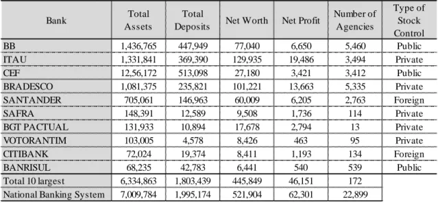
agencies. In 2016, there were 174 banks and 22,547 banking agencies. Table 2 presents
the ten largest banks in 2016, with their total assets, total deposits, net worth, net profit,
number of agencies and type of stock control.
Table 2: The 10 largest banks in Brazil, 2016 (R$ 1,000,000)
Source: FEBRABAN (2016)
In the 1990s, Brazil began a process of opening commercial and financial markets
to foreign transactions. Foreign banks increased their participation in the Brazilian market
and mergers and acquisitions intensified. However, foreign banks maintained a
conservative strategy that contributed little to the expansion of credit concessions, spread
reduction, or quality and diversification of financial products and services.
Even with the entry of international banks, the cost of capital, which is determined,
among other factors, by the interest rate, the SELIC rate, and by the spread fixed by the
banks, has remained excessively high.
In this way, the financial system is characterized as dysfunctional or of low
macroeconomic efficiency, due mainly to the existing incentives: on the asset side,
Bank Total
Assets
Total
Deposits Net Worth Net Profit
Number of Agencies
Type of Stock Control
BB 1,436,765 447,949 77,040 6,650 5,460 Public
ITAU 1,331,841 369,390 129,935 19,486 3,494 Private
CEF 12,56,172 513,098 27,180 3,421 3,412 Public
BRADESCO 1,081,375 235,821 101,221 13,663 5,335 Private
SANTANDER 705,061 146,963 60,009 6,205 2,763 Foreign
SAFRA 148,391 12,589 9,508 1,736 114 Private
BGT PACTUAL 131,933 10,894 17,678 2,794 13 Private
VOTORANTIM 103,005 4,578 8,426 463 95 Private
CITIBANK 72,024 19,374 8,411 1,193 134 Foreign
BANRISUL 68,235 42,783 6,441 540 539 Public
investments in government bonds and on the liabilities side, raising funds from middle
and high cost agencies.
Private banks display higher concentration of short-term operations, investments
in securities and investments in securitization. Public banks dedicate a greater proportion
of resources to credit operations.
Camargo (2009) highlights some of the characteristics of the banking sector in last
decade:
i) Banks act as financial intermediaries, with bond markets playing an almost irrelevant role in financing private activity;
ii) A high degree of concentration in the banking sector;
iii) The structure of the banking sector encourages the emergence of a form of oligopolistic competition, in which leading banks set the basic prices of financial services and compete with each other through service differentiation rather than price;
iv) The performance of non-leading banks in niches not attractive to the leading banks, due to the few conditions for the former to exert more effective competitive pressures on the latter in the more attractive markets;
v) The permanent situation of economic instability and fiscal deficits, which led successive governments to offer large amounts of government bonds, under extremely favorable conditions of return and liquidity.
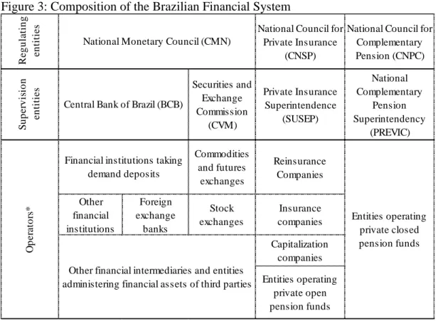
Financial institutions in Brazil are ruled by the National Monetary Council (CMN)
and supervised by the BCB. Figure 3 presents the composition of the Brazilian financial
system.
The current economic system in Brazil, called the “Real Plan”, began in 1994.
Before this date, Brazil experienced a high inflation rate. The “Real Plan” met three steps
to access price stability: i) a fiscal adjustment (May 1993 to February 1994); ii) monetary
reform (March to July 1994) and iii) the adoption of an anchor exchange rate (July 1994
to January 1999).
Since 1999, the Inflation Target Regime (RMI) has been adopted. The Monetary
Policy Committee (COPOM) was created on June 20th 1996, and was assigned the
responsibility of setting the stance of monetary policy and the overnight interest rate
(SELIC rate). The BCB ensures that the target of the SELIC rate works, through open
Figure 3: Composition of the Brazilian Financial System
Source: Central Bank of Brazil (2017)
The COPOM publishes a report, eight times a year, since 1998. In this report it
describes the economic conditions (inflation behavior), risks around inflation, and a
discussion around monetary policy conduction.
In the last decade, the inflation target is being achieved. Between 2004 and 2014
the observed inflation expressed in the General Consumer Prices Index (IPCA) stayed
below the upper goal limit, except in 2015, when observed inflation was above the target.
In 2014 and 2015, the SELIC rate showed an increase. However, in December 2017, the
observed inflation rate was considered smaller than expected and the SELIC rate was
fixed at 7% (BCB, 2017), decreasing from 14.15% in December 2015, the highest interest
rate of the decade.
Despite the success in controlling inflation since its implementation in Brazil, the
economy's performance was below expectations. The total GDP reveals a recession in the
Brazilian economy. The GDP increased, on average, 4.8% between 2004 and 2008;
decreased 0.1% in 2009, increased, on average, 4% between 2010 and 2013; increased
just 0.5% in 2014; and decreased, on average, 3.8% in subsequent years. The evaluation
of fixed investments in the last decade shows a movement synchronized to GDP: a high
decrease in 2009, in 2014 and in subsequent years (IBGE, 2017).
R e g u la tin g e n titie
s National Council for
Private Insurance (CNSP)
National Council for Complementary Pension (CNPC) S u p e rv is io n e n titie
s Securities and
Exchange Commission (CVM) Private Insurance Superintendence (SUSEP) National Complementary Pension Superintendency (PREVIC) Commodities and futures exchanges Reinsurance Companies Other financial institutions Foreign exchange banks Stock exchanges Insurance companies Capitalization companies Entities operating private open pension funds National Monetary Council (CMN)
Central Bank of Brazil (BCB)
O p e ra to rs *
Financial institutions taking demand deposits
Entities operating private closed pension funds
3.1 Methodology
The FOF analyses was used to provide evidence of the financial structure of
Brazilian economy and investigate relationship between the objective economy and the
financial economy. Two sets of ALM (and ALM*) were developed: one from 2004 to
2009 and another from 2009 to 2014.
Dispersion indexes were calculate and combined as follows: i) the PDI-FR and
PDI-FE give the position of the institutional sectors in the financial market and the
financial intermediary—it usually shows both a DPI close to 1 and the highest indexes
indicating a better ability in borrowing and lending funds; and ii) the FR and
SDI-FE that are used to measure the importance of each sector as intermediaries in the
financial market (how they react to changes in total demand of funds).
The evolution of the power-of-dispersion and sensitivity-of-dispersion indexes
were observed to investigate if there was any changes in the behavior of institutional
sectors in the financial market.
Furthermore, the discrepancy index was calculated to the years 2004 to 2014. For
2008 and 2013 a decomposition of the change in discrepancy is made, and present an
expanded ALM to the year 2009, in which financial institutions are disaggregated, is
presented.
3.2 Brazilian Data
The data used to apply the FOF analysis in the Brazilian economy are the Financial
Balance Sheet of Brazil and the balance sheet of the BCB. The balance sheets of the BCB
are available on the BCB web site.
For the period 2004–2009, the Financial Balance Sheet of Brazil is available from
the Brazilian Institute of Geography and Statistics (IBGE)5. For the period 2009–2014, it
is available from the Organization for Economic Co-operation Development (OECD).
The financial balance sheet is an accounting statement that presents the stock of
financial assets and liabilities held by economic agents in a beginning date, the variations
that occurred in these assets and liabilities during the period of one year and the assets
and liabilities held in the final date of ascertainment of the balance sheet. This financial
5 IBGE is official organization responsible to collect, organize and publish information and data to
balance sheet was published for the years 2004 to 2009 as a part of the Integrated
Economic Accounts (CEI) by the BCB, together with the IBGE.
After 2009, the publication was discontinued publication and then it was available
from the OECD for the period 2009–2014. The non-consolidated SNA 2008 is used
(OECD, 2018).
The financial assets and liabilities are detailed in seven main financial instruments
held by five institutional sectors: non-financial firms, financial firms, households,
government and the rest of the world (ROW)7. Below, the main financial instruments are
listed:
F1. Gold and DES* F2. Cash & Deposits F3. Bonds
F4. Loans F5. Shares
F6. Technical insurance F7. Others
*Gold and DES are not included in FOF BR because they refer to monetary funds.
The “financial enterprises” were disaggregated into two subgroups: the central
bank and “other financial enterprises,” subtracting the flows of assets and liabilities of the
BCB (obtained from its balance sheet) from the flows of financial assets and liabilities of
the “financial enterprises” in the financial balance sheet.
The balance sheet of the BCB is published monthly together with other financial
statements and explanatory notes. Was used the annual data related to the exercises closed
in December 31th of each year between 2004 and 2014. The balance sheet is an
accounting statement that represents stock accounts, indicating the stock of assets
(physical and financial assets) and liabilities (obligations and equity) held by an entity on
a certain date. The elaboration of the balance sheet of the BCB follows the Central Bank’s
General Accounting Plan (PGC). The balance sheet of the BCB has been available
monthly from 1965 until 2017. Figure 4 presents the BCB balance sheet structure.
Figure 4: Accounting Structure of the Balance Sheet of Central Bank of Brazil
Source: Financial Statements (BCB, 2017)
For 2008 and 2009, an additional disaggregation of financial firms was made. The
“other financial enterprises” were disaggregated into four financial institutions: three of
them are government-sponsored financial institutions—Banco do Brasil (BB), Caixa
Econômica Federal (CEF), and Banco Nacional de Desenvolvimento Econômico e Social
(BNDES)—and one is the largest private bank, in terms of total assets in Brazil, the Itaú
Bank. All of these financial institutions play important roles in the Brazilian economy.
The assets and the liabilities of these institutions, presented in their balance sheets,
were subtracted from the flows of “other financial enterprises”. The financial statements
of the financial institutions operating in Brazil are published monthly by BCB. Their
structures follow the Financial Institutions Accounting Plan (COSIF), which follow the
PGC. Was used the annual data related to the exercises closed in December 31th of each
year from 2004 to 2009.
1.ASSET 2.LIABILITY 1.1.FOREIGN CURRENCY ASSETS 2.1.FOREIGN CURRENCY LIABILITIES 1.1.1.Available 2.1.1.Contracted operations to be settled 1.1.2.Time deposits in financial institutions 2.1.2.Deposits in financial institution 1.1.3.Resale agreement 2.1.3.Repurchase agreement
1.1.4.Derivative 2.1.4.Derivatives
1.1.5.Securities 2.1.5.Credits to pay
1.1.6.Credits Receivable 2.1.6.Deposits in International Financial Organization 1.1.7.Gold 2.1.7.Other
1.1.8.Participation in International Financial Organization
1.1.9.Other 2.2.LOCAL CURRENCY LIABILITIES 2.2.1.Contracted operations to be settled 1.2.LOCAL CURRENCY ASSETS 2.2.2.Deposits from financial institution 1.2.1.Available 2.2.3.Repurchase agreement
1.2.2.Deposits 2.2.4.Derivatives
1.2.3.Resale agreement 2.2.5.Liabilities with federal government
1.2.4.Derivative 2.2.6.Credit to pay
1.2.5.Federal public securities 2.2.7.Deposits in International Financial Organization 1.2.6.Credit with federal government 2.2.8.Provisions (Allowance)
1.2.7.Receivable credit 2.2.9.Other 1.2.8.Bens Móveis e Imóveis
1.2.9.Other 2.3.CIRCULATING 2.4.NET WORTH 2.4.1.Result Reservation 2.4.2.Revaluation Reserve
2.4.3.Unrecognized gains / losses in income 2.4.4.Effects of Changes in Accounting Practices 2.4.5.Accumulated result
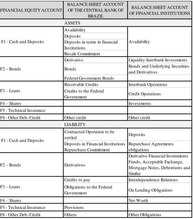
A “Plan of Codification” was made to link the asset and liability accounts of the
BCB, the financial institutions’ balance sheets, and the financial instruments of the
financial balance sheets from the PGC, COSIF and the Methodological Notes of financial
balance sheet (IBGE, 2011). The “Plan of Codification” proposed is presented in Table
3.
Table 3: Plan of Codification between Financial Instruments in the Financial Equity Account, Balance Sheet of the Central Bank and the Balance Sheet of Financial Institutions
Source: Elaborated by authors FINANCIAL EQUITY ACCOUNT
BALANCE SHEET ACCOUNT OF THE CENTRAL BANK OF
BRAZIL
BALANCE SHEET ACCOUNT OF FINANCIAL INSTITUTIONS
ASSETS Availability Deposits
Deposits in terms in financial Institutions
Resale Commitment
Derivative Liquidity Interbank Investments
Bonds Bonds and Underlying Securities and Derivatives
Federal Government Bonds
Receivable Credits Interbank Operations Credits to the Federal
Government Credit Operations
F4 – Shares Investments
F5 - Technical Insurance
F6 - Other Deb./Credit Other credit Other credit LIABILITY
Contracted Operation to be
settled Deposits
Deposits in Financial Institutions Repurchase Commitment
Repurchase Agreements obligations
F2 – Bonds Derivatives
Derivative Financial Instruments Funds, Acceptable Exchange, Mortgage Notes, Debentures and Similar
Credits to pay Interdependence Relations
Obligations to the Federal
Government On Lending Obligations
F4 – Shares Net Worth
F5 - Technical Insurance Provisions
F6 - Other Deb./Credit Others Other Obligations F3 – Loans
F1 - Cash and Deposits Availability
F2 – Bonds
F3 – Loans
4. Brazilian Flow-of-Funds
Tables 4 and 5 presents the asset table (E-Table) and liability table (R-Table),
respectively, from the Flow of Funds Account 2005. The main bloc of accounts in Table
4 represent the amount of funds that the institutional sector employed to each financial
instrument in terms of all of the asset investments or the portfolio investment of each
sector. These elements were defined in Equation 1: ��� . The row “Diff. (Excess Liability)”
expresses the excess of liabilities. Looking at each sector, the difference observed on its
balance sheet reveals whether this sector has a net financing capability (net lending)
which means a savings excess in the real economy. In Equation 1, it was referred to vector
ε�. In this same equation, the total of the instruments in terms of assets (vector ���) is
shown in the last column of Table 4 and the total of resources of each sector (vector �� -
the last row in Table 4.)
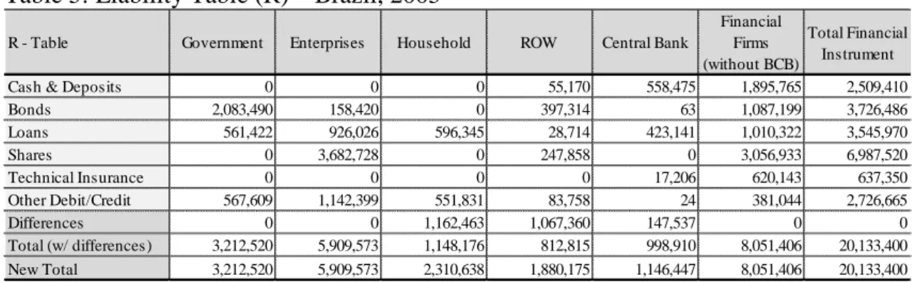
The main bloc of accounts in the R-Table (Table 5) are elements that represents
the amount of funds the sector has raised from each financial instrument, representing all
of financial liabilities used by this sector (the liability portfolio or capital structure of the
institutional sector). The elements of R-Table described in Equation 2 are highlighted in
Table 5. The row “Diff. (Excess Assets)” represents vector ρ�, which expresses the excess
of assets related to those sources of funds. In the real economy, it indicates which
institutional sector has an investment excess or net financing necessity (net borrowing).
The last column in Table 5 represents the vector ���, which is the sum of liabilities. The
last row in Table 5 represents the vector ��, which refers to the total financial funds of
each sector.
Tables 6 and 7 present the ALM in the liability-oriented system and in the
asset-oriented system, respectively defined as Y and Y*. The sectors are in rows and columns,
and the intersections represent the flow of funds between institutional sectors. Table 6
presents the amount of funds the sector in the column raises from the sector in the row.
Table 7 presents how many funds the row sector applied to the column sector (current
Table 4: Asset Table (E) – Brazil, 2005
Source: Elaborated by authors from the Flow of Funds Account
Table 5: Liability Table (R) – Brazil, 2005
Source: Elaborated by authors from the Flow of Funds Account
Table 6: Asset–Liability Matrix in the Liability System (ALM), Brazil 2009
Source: Elaborated by authors
Table 7: Asset–Liability Matrix in the Asset System (ALM*), Brazil 2009
Source: Elaborated by authors
E - Table Government Enterprises Household ROW Central Bank
Financial Firms (without BCB)
Total Financial Instruments
Cash & Deposits 847,761 419,489 459,699 9,060 32,952 740,449 2,509,410 Bonds 72,176 225,844 192,536 298,572 1,026,191 1,911,169 3,726,486 Loans 652,978 52,543 12,942 175,061 83,849 2,568,596 3,545,970 Shares 393,492 2,646,984 777,222 1,244,980 0 1,924,842 6,987,520 Technical Insurance 292 10,150 623,211 738 0 2,958 637,350 Others Deb./Credit 677,911 1,194,021 245,027 151,765 3,455 454,486 2,726,665
Differences 567,910 1,360,543 0 0 0 448,908 0
Total (w/ differences) 2,644,611 4,549,030 2,310,638 1,880,175 1,146,447 7,602,499 20,133,400 New Total 3,212,520 5,909,573 2,310,638 1,880,175 1,146,447 8,051,406 22,510,760
R - Table Government Enterprises Household ROW Central Bank
Financial Firms (without BCB)
Total Financial Instrument
Cash & Deposits 0 0 0 55,170 558,475 1,895,765 2,509,410 Bonds 2,083,490 158,420 0 397,314 63 1,087,199 3,726,486 Loans 561,422 926,026 596,345 28,714 423,141 1,010,322 3,545,970
Shares 0 3,682,728 0 247,858 0 3,056,933 6,987,520
Technical Insurance 0 0 0 0 17,206 620,143 637,350
Other Debit/Credit 567,609 1,142,399 551,831 83,758 24 381,044 2,726,665
Differences 0 0 1,162,463 1,067,360 147,537 0 0
Total (w/ differences) 3,212,520 5,909,573 1,148,176 812,815 998,910 8,051,406 20,133,400 New Total 3,212,520 5,909,573 2,310,638 1,880,175 1,146,447 8,051,406 20,133,400
Sector Government Enterprises Household ROW Central Bank Financial
Firms Total Government 6,878,877 6,495,426 1,467,414 891,357 1,314,281 8,986,602 26,033,958 Enterprises 5,790,401 17,660,747 2,273,263 1,506,109 1,804,644 14,706,529 43,741,692 Household 3,116,944 5,647,588 3,441,557 785,281 1,041,691 8,239,550 22,272,612
ROW 2,444,552 4,826,780 895,471 2,513,054 726,561 6,040,189 17,446,608
Central Bank 1,994,384 2,550,253 550,682 454,312 1,631,186 3,708,043 10,888,861 Financial Firms 10,989,200 18,525,175 4,000,611 2,632,583 3,454,753 33,068,494 72,670,817 Total 31,214,360 55,705,970 12,628,999 8,782,696 9,973,116 74,749,407
Sector Government Enterprises Household ROW Central Bank Financial
Firms Total Government 6,878,877 5,790,401 3,116,944 2,444,552 1,994,384 10,989,200 31,214,360 Enterprises 6,495,426 17,660,747 5,647,588 4,826,780 2,550,253 18,525,175 55,705,970 Household 1,467,414 2,273,263 3,441,557 895,471 550,682 4,000,611 12,628,999
ROW 891,357 1,506,109 785,281 2,513,054 454,312 2,632,583 8,782,696
Overall, the tables show that households employ funds mainly in the form of
shares, “other credit” and insurance technical reserve and their ratio of cash & deposits is
relatively low. Shares include listed stocks and shares in investments funds (the largest
portion) and insurance technical reserve includes life insurance and pension funds. Most
of these financial instruments are available from financial institutions.
Moreover, “other credit” includes trade credit and advances. The high ratio of
other credit together with the low ratio of cash & deposits indicate there is a huge amount
of informal financial activity.
Non-financial firms are raising funds mainly through shares (between 50% and
60% of their capital structure). Treasury bonds (i.e., bonds issued by the government) are
the main fund-raising instruments of the government (e.g., 62.0% in 2004 and 64.9% in
2009). The ALM reveals that these funds come from foreign funds, from BCB, and from
financial institutions, which have increased their employment of funds in governments
bonds.
To begin the analyses, the FOF Leontief inverse was obtained, from which the
FOF indexes were extracted. The discrepancy index revealed two important changes: i)
two dates when there was a “collapse” in the financial system (in 2008 and 2013); and ii)
one date when there was a change in the signal of discrepancy (2010).
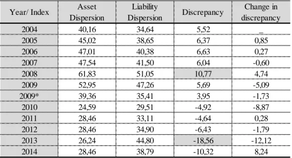
Table 8 presents the asset dispersion, liability dispersion and discrepancy of
dispersion to Brazilian FOF from 2004 to 2014 (obtained with Equations 17 to 19).
Table 8 shows two years (2008 and 2013) with a higher discrepancy of dispersion.
These high discrepancies occur in different contexts, in 2010, there was a modification in
the sign of the discrepancy index and the total sum of the Leontief inverse in the asset
system became smaller than in the liability system. This context extended to the following
years. Looking at the asset table and the liability table (E, R) together, it is observed that
in a wide economy there are excess assets and the amount of savings are greater than the
amount of fixed investments in the objective economy until 2010. After 2010, there is
excess liability in the financial system, which means savings are smaller than investments
Table 8: Asset dispersion, liability dispersion and discrepancy of dispersion, Brazil, 2004 to 2014
* The two set of Brazilian ALM include the year 2009. Source: Elaborated by authors.
Around 2007, there was a rumor of an international financial crisis. Institutional
sectors, i.e., entrepreneurs, for fear of making physical investments, responded with an
increase in interest rates, and excess savings accumulated in the financial system.
The year 2008 was the crucial point where the growth in excess assets was so great
that it caused a high discrepancy index (concomitant to Lehman Brothers bank
breakdown). In the next year, 2009, the Brazilian GDP effectively fell.
In 2009 and in subsequent years, CMN adopted set of anti-cyclical measures, as
well as fiscal, monetary and credit policies. The effect was a change in the financial
behavioral in the economy, and since 2010, there has been a change in the signal of
discrepancy of dispersion. Meanwhile, the remedy was excessive, and in 2013 there was
another collapse in the financial system; however with excess liabilities this time and at
the same time, it is observed an increase in the interest rate. As a consequence, the GDP
of 2014 shows a decrease in the growth rate and in the subsequent years (2015 and 2016)
the GPD effectively decrease. Figure 5 presents the evolution of the SELIC rate, the
discrepancy dispersion and the change in GDP from 2009 to 2014.
The structure of the Brazilian financial market, illustrated by
power-of-dispersion-index fund-raising and fund-employment, shows that households and the ROW are
mainly “saving sectors” (the DPI-FE is higher than the DPI-FR). They are saving and
accumulating financial assets. Meanwhile, enterprises and government are mainly
“investor sectors” (the DPI-FE is lower than the DPI-FR); they usually raise funds to
Year/ Index Asset
Dispersion
Liability
Dispersion Discrepancy
Change in discrepancy
2004 40,16 34,64 5,52 _
2005 45,02 38,65 6,37 0,85
2006 47,01 40,38 6,63 0,27
2007 47,54 41,50 6,04 -0,60
2008 61,83 51,05 10,77 4,74
2009 52,95 47,26 5,69 -5,09
2009* 39,36 35,41 3,95 -1,73
2010 24,59 29,51 -4,92 -8,87
2011 28,46 33,11 -4,64 0,28
2012 28,46 34,90 -6,43 -1,79
2013 26,24 44,80 -18,56 -12,12
finance excess investments in the objective economy. The Brazilian Central Bank is in
the middle of the financial market, while other financial firms are a little below, which
means that they have more difficulty employing funds.
In the first part of the period 2004–2009, these indexes are interesting in pointing
out that the government and the central bank take on more important roles, with greater
influence in the financial market, over financial firms (the financial sector without the
central bank). The government borrows new sources of financing by issuing treasury
bonds and/or borrowing new loans and BCB provides funds to ultimately finance the
needs of all other financial institutions as well as the government's deficits. This
highlights the great power of the government and the central bank in the Brazilian
economy and raises a question in relation to their financial intermediation performance.
Figure 5: SELIC rate, Discrepancy dispersion and GDP Change, Brazil, 2009 to 2014
Source: IBGE; BCB and Brazilian FOF
The BCB has low SDI-FE, indicating that it does not immediately react to savings
increases. However, the financial firms, government and enterprises are strongly
influenced by increases in total savings.
In this sense, enterprises and the government seem to work as financial
intermediaries, because they generate great influence when borrowing and are strongly
affected when there are excess investments in the wide economy.
The evolution of the power of dispersion indexes from 2010 to 2014 shows that
the household and enterprise sectors are moving toward the middle (1, 1), indicating that
ROW stays in the second quadrant, near households, and plays an important role as a
supplier of funds.
The government stays in the fourth quadrant, proving that its role in the financial
market is not much different from that of enterprises; the government is actively investing.
Financial firms are still situated in the fourth quadrant, indicating that they are better at
borrowing than lending.
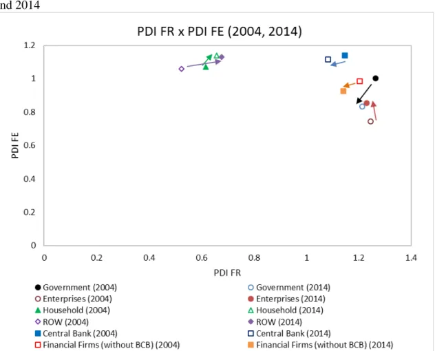
Figure 6 plots the graphics with the power-of-dispersion-indexes from the year
2004 to 2014. The FR assumes values in the abscissa (horizontal axis) and the
DPI-FE in the ordinate (vertical axis). The center of the graphic assumes the value of 1.
Figure 6: The position shifts of institutional sectors in the PDI diagram, Brazil, 2004 and 2014
Source: Elaborated by authors
Households moved a little north-east in the diagram, suggesting the sector has
become a dominant player as a funds supplier. Similar, although more intense, movement
is observed in the rest of world, implying that Brazilians are finding their investment
Enterprises moved northward, implying that their presence as a fund supplier rose
during the observation period.
The government moved to the south-west, suggesting that the private sector has
taken over the economic dominance.
Figure 7 plots the graphics with the power-of-dispersion-indexes from the year
2004 to 2014. The FR assumes values in the abscissa (horizontal axis) and the
SDI-FE in the ordinate (vertical axis). The center of the graphic assumes the value of 1.
Figure 7: The position shifts of institutional sectors in the SDI diagram, Brazil, 2004 and 2014
Source: Elaborated by authors
Looking at the sensitivity-of dispersion-indexes, financial firms stay in the first
quadrant and their position is moving toward the right, suggesting that there is
considerable improvement in their performance as intermediaries.
As a consequence, the financial firms can absorb the household savings more
effectively; households moved eastwards in the diagram from the third quadrant to the
Enterprises and the government moved to south-west, implying that they are no
longer active as financial intermediaries.
On the other hand, the central bank and the government move left, showing that
their role as intermediaries is decreasing. Notwithstanding, enterprises are situated in the
first quadrant, suggesting trade credit is an essential tool of finance in Brazil.
According to the order of the SDI-FRs, individuals tend to borrow first with
financial firms (which means the financial system without the central bank), then with
enterprises and then from the government.
Figures 8 and 9 present the fluctuations in FR-PDI from 2004 to 2009 and from
2009 to 2014, respectively.
Households’ FR-PDI significantly rose in 2008 and showed a moderate rise in
subsequent years. From 2008, the mortgage and consumer-finance market was heated in
Brazil because of anti-cycle polices as a consequence of the credit crunch. As well as
households’, the rest of world’s FR-PDI significantly rose in 2008, however the index
dropped in 2009 and 2010.
Enterprises, government, financial firms, and the BCB’s FR-PDI show a
downward trend, although the enterprise sector showed a small growth in 2010.
Figure 8: Fluctuation of institutional sectors in DPI-FR, Brazil, 2004–2009
Figure 9: Fluctuation of institutional sectors in DPI-FR, Brazil, 2009–2014
Source: Elaborated by authors
Figures 10 and 11 presents the fluctuations in FE-PDI from 2004 to 2009 and from
2009 to 2014, respectively.
Figure 10: Fluctuation of institutional sectors in DPI-FR, Brazil, 2004–2009
The government’s and central bank’s FE-PDI declined significantly in 2008 while
the ROW and financial firms’ indexes grew. In the previous year, there was an excess
inflow of financial funds from abroad, as observed in the discrepancy indexes, there were
excess assets in the economy. However, funds were almost all concentrated in financial
firms, not allocated to productive sectors.
Figure 11: Fluctuation of institutional sectors in DPI-FR, Brazil, 2004–2009
Source: Elaborated by authors
Financial firms’ FE-PDI dropped sharply in 2010, while the government and the
central bank’s FE-PDI rose, suggesting that the credit crunch was triggered by the
reluctance of banks to extend new loans; instead, the government and central bank took
on anti-cycle politics to help the economy out of the crisis.
Figure 12 presents the fluctuations in FR-SDI from 2009 to 2014 and Figure 13
presents the fluctuations in FE-SDI from 2009 to 2014. Figure 12 reveals that financial
firms absorbed most of the fluctuations in the demand for funds in the Brazilian economy.
However, financial firms’ FR-SDI dropped sharply in 2010, showing that the credit
crunch was a factor. Moreover, it should be noted that the FR-SDI of the government and
central bank dropped one year earlier; the credit crunch must have been caused by
Figure 12: The fluctuations in FR-SDI, Brazil, 2009–2014
Source: Elaborated by authors
Figure 13: The fluctuations in FE-SDI, Brazil, 2009–2014
The rise in households’ FR-SDI suggests that the fund raisers found a last resort
in the sector. Another problem is that the rest of world’s FR-SDI declined sharply in
2013; the exchange rate had been in a growth trend since 2011. In 2012, 2013, and
2014, the growth rate was 13% each year, which could have generated distortions in
imports and exports.
Figure 13 shows that the FE-SDI of enterprises rose while that of the central
bank dropped in 2009, suggesting that enterprises mutually gave credit among them to
continue their day-to-day business under economic tightening.
The dispersion indexes in the years 2008, 2009, and 2010 that a lot of changes
occurred in the behavior of institutional sectors in the financial market. Remembering
that according to discrepancy index, the year 2008 was a crucial year, demonstrating
higher discrepancy.
Figure 14 presents a diagram of the Brazilian financial system with the additional
disaggregation in the financial firms (for BCB and the three government-sponsored
financial institutions: BB, CEF, and BNDES; Itaú Bank, the largest private bank; and the
group of “other financial firms”). It shows FR-PDI and FE-PDI in the year 2009. Figure
15 shows FR-SDI and FE-SDI to this additional disaggregation.
The wide view presented in Figure 14 shows that BB, CEF, and BNDES are higher
than “other financial firms” and the private bank, indicating that government-sponsored
banks showed greatest ability to spreads funds. However they did not showed ability to
absorb changes in demand. Figure 15 reveals that other financial firms have the ability to
absorb demand (they are in the upper and right side of the graph) than
government-sponsored banks.
Therefore, one part of the demand for funds is supplied by “other financial firms,”
who do not effectively pass on these funds and the other part of the demand is supplied
by the informal market.
In the next sequence, the decomposition of change in the discrepancy of dispersion
is presented. Table 9 presents the decompositions of the change in the discrepancy index
within the contributions of the objective economy and contributions of the financial
Figure 14: The position of financial firms in the PDI diagram, Brazil, 2009
Source: Elaborated by authors
Figure 15: The position of financial firms in the SDI diagram, Brazil, 2009