Finite Element Approach for Schrodinger Equation with Lennard-Jones Potential
* **
Hideyuki Arai, Isao Kanesaka and Yukio Kagawa
(October 1975)
Finite element approach is successfully applied to-the vibrational Schrodinger equation
with Lennard-Jones potential. Ar, atom molecules are considered for diatomic problem, for which the eigen values, the corresponding eigen functions and the vibrational level spacings are calculated.
The cal cui a ted values agree with those experimental! v obtained. This verifies the validity of the present approach, which paves the way to the application to the prr1blems of this kind.
Introduction
Finite Element Method was originally developed for the analysis of structures and have now wi
dely been applied to various classes of problem in engineering science because of its versatility.
Among others the method is successfully applied to the analysis of the field problems, of Laplace, Poisson and Helmholtz equation.1l,2l The Finite Element Method is a variant of Rayleigh-Ritz pro
cedure and a process to discretize the continuum field with the best possible approximation by means of the variational calculus which minimizes the functional corresponding to the governing differential equation. Therefore the present procedure can be said to be an extended approach of the variational calculus which has intensively been utilized in wave mechanics. 3)
The purpose of this paper is to present the finite element technique for the vibrational Schrodinger equation with two body potential V which is expressed as follows:
d' rj; 2!1 (l)
dW' + h'(E-Vlrf;=U
where rf; is a wave function, Q a normal coordinate, J1 a reduced mass, and E an eigen value.
If V is expressed by
V(Q) = � 1 KQ' 2
(2)
where K is a force constant. Equation (1) is known as the Schrodinger equation of harmonic oscil
lator and can be solved precisely.
ln case of Lennard-Janes potential, 4) V is expressed as:
(3)
where c: is a potential energy in equilibrium distance r, and q a distance of two bodies at V = c:.
The eigen values and their associated wave functions for harmonic oscillators as well as those under the Lennard-Janes potential are numerically calculated by means of flement element approach.
The results are compared with those obtained analitically and experimentally.
II. Functional and Finite Element Formulation
Plccording to the variational calculus the solution of equation (6) is equivalent to finding the fu
nction ¢which minimizes the following functional: 3)
� { 1 (a¢') 1 211-
, }
x= Q -2 -- - --(E -V)rp dQ aQ 2 h2 (4)
which physically corresponds to the expectation value in quantum theory. The integration 1s taken over the whole region under consideration.
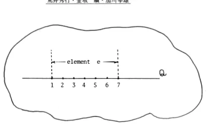
The region in which the problem is to be solved is divided into small elements as shown in Figurel, for which the trial function is assumed to be
(5)
where the components of N are spatial function and the a, are seven unknown constants to be chosen so as to satisfy the nodal values at the element nodes.
Thus the function ¢ is uniquely specified within the element by the nodal values¢1,¢2,¢3, • • • • ,¢, and their associated coordinates as
l¢'"'1�
e
:}
I al �c'"' I al (6)( ) {e)
where ( J e refers to the element. I ¢ \ indicates the values of ¢ at the element nodes, which is
where T denotes the transpose, and N, consists of the coordinate values corresponding to node ·i , which is
N,= \1 Q, Q� Q7···Q!-1 I
- 2 -
C(ef1. (e) .
Premultiplying the each side of the equation (6' by (mverse of C matr.1xl and substituting ja\
into equation (5 ', we obtain the trial function as
Substituting equation (71 into equation (41 the functional for the element is given by where
( ) 1 T -IT ( ( ) -!
X e =-1 rj}e)l (C (e)J (A� EB e J C (ej 1 r/J(e)l 2
B (e) -'!:..!!_I h2 e NTNdQ
where the integration is taken over the element.
(el
(7)
(8)
(9) (10)
To minimize the functional X, we take the partial derivative with respect to I </1 I and to give
(11)
Equation (ll) holds for all the elements that divide the space.
The values of ¢,. at the interconnecting nodes between abjoining elements must be the same. With this compatibility imposed, we obtain linear algebraic equation of the form
(A- EB)l ¢ I = o (12)
The eigen values and the wave functions are calculated from equation (12).
III. Numerical Examples
The functional of equation (4) is defined in unbounded space, for which the integration must be carried out. This can not be achieved in numerical analysis. Since the lower eigen values are gener
ally of our interest, the potentialdistribution is first calculated for which the region where the potential forms the well are divided into the elements.
The fir st examples of the calculation are the harmonic oscillators of hydrogen and oxygen. That is, equation (1) is to be solved under equation (2), which can analytically be solved.
The sixth order polinomial 1s used as the trial function of the element, Six elements divide the region to be integrated which is chosen so as to cover the lowest some eigen values. Two schemes are considered for the way of division:
Case 1. Equal space division.
Case 2. Finer division are employed in the vicinity of the potential well.
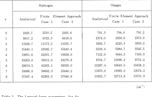
The calculated lowest eight eigen values are shown in Table 1. The values obtained by the finite element approach reasonably agree with the analytical ones. The results are not free from the way
of the computer used. The present approach is, however, promissing if proper way of division is cho
sen ( Case 2). Figure 2 shows the potential distribution and the eigen functions (which are not normalizE in the figure) corresponding to the lowest six eigen values.
The next examples of calculation are for the case of Lennard-Jones potential. lt is to solve equa
tion ( 1) under equation ( 3). Argon molecules are considered, for which the experimental values of the vibrational level spacings are already given.151 Lennard-Jones parameters are given in Table 2,
from which the potential of equation (31 is calculated. The region where the potential is negative is chosen for integration. The order of the pol inomial of the trial function and the number of the division are the same as above. Finer division is used in the vicinity of the potential well !Case 2).
The calculated vibrational level spacings and their experimental counterparts are shown in Table 3.
Reasonable agreement is again obtained.
ln Figure 3, the potential distribution and the eigen functions for argon molecules in the Len
nard-Janes potential are also shown. The dotted lines for the eigen functions are hypothetically drawt), as they are out of the region of integration.
N. Final Remarks
Finite element approach is successfully applied to the vibrational Schrodinser equation.
ln the present paper, some simple examples of diatomic molesule problems are considered for the verification of the i).pproach.
The Finite Element Method is promissing and paves the way to the application to the wide range of the problems of this kind.
The numerical calculation was performed at Toyama University Computer Center.
References
(1) O. C. Zienkiewicz, " The Finite Element Method in Engineering Science", McGraw-Hill, London
( 1971).
(2) Douglas H. Norrie and Gerard de Vries, " The Finite Element Method", Academic Press, New York and London (1973)
(3) Leonard I. Shiff, "Quantum Mechanics", McGraw-Hill, London (1968).
(4) P. A. Egelstaff, " An Introduction to the Liquid State", Academic Press, New York and London
(1967) (5) Kate K. Docken and Trudy P. Schafer, "Spectroscopic Information on Ground-State Ar,, Kr, and Xe2· from Interatomic Potentials", Journal of Molecular Spectroscopy, 46, 455-459 (1973).
- 4 -
Table 1. The eigen values for the harmonic oscillator of the diatomic molecules
Hydrogen
Finite Element Approach
v Analytical Analytical
Case 1 Case 2
0 2205.7 2210.2 2205.6 791.3
1 6617.2 6725.3 6618.6 2374.0
2 11028.7 11172.2 11035.7 3956.7
3 15440.1 16585.7 15449.4 5539.4
4 19851.6 22291.7 19838.0 7122.0
5 24263.0 39015.9 24276.8 8704.7
6 28674.5 42265.1 28925.0 10287.4
7 33086.0 58842.3 33440.2 11870.0
8 37497.4 62265.5 37946.8 13452.7
Table 2. The Lennard-Jones parameters for Ar,
E a
(cm·1) cA..)
Ar 2 115.1 3.35
Table 3. The eigen values for Ar2 in the Lennard-Jones pottential
vibrational level spacings
v Experimental Finite Element Approach
0 25.0- 26.7 23.74
1 18.6- 20.8 18.97
2 14.8- 16.2 14.55
3 9.2- 11.3 9.81
4 5.9- 8.0 8.47
Oxygen
Fini te Element Approach Case 1 Case 2
794.0 791.2 2458.6 2373.9 4220.3 3959.0 5984.7 5545.5 9444.3 7169.9 10996.2 8751.4 16649.0 10434.2 19385.0 12074.3 22713.8 13731.9
' I
�-element
I ' '
e-I
1 2 3 4 5 6 7
Figure.! Division of a region into elements.
0
,...._ -20
...
' 0
,.,..
0 ...
� '"' Q) [i
...
"' ...
.., [i
.., 0 0..
2
-0.12 0.0 0.12
A .
Normal coordinate Figure 2.
The potential fWlction and the calculated eigen fWlctionsfor the harmonic oscillator of oxygen molecule. The solid horizontal lines show the level of the eigenvalues.
&"' le
�
@ !-<
... �
"' ...
� ..,
&
- 6- -40
-60 -so
-100
-120
3.0 4.0 5.0 6.0
Atomic distance (A)
Figure 3. The potential function and the calculated ei�en functions (arbitrary unit) of the Ar2 molecule.
The solid horizontal lines show the level of the eigen values. The dotted lines are hypothetically drawn.