Instructions for use A uthor(s ) S abau,S orin V ; S himada,Hideo
C itation Hokkaido University Preprint S eries in Mathematics, 835: 1-29
Is s ue D ate 2007
D O I 10.14943/83985
D oc UR L http://hdl.handle.net/2115/69644
T ype bulletin (article)
F ile Information pre835.pdf
Sorin V. Sabau and Hideo Shimada
Dedicated to the memory of Professor Makoto Matsumoto
Abstract. This paper study the Gauss-Bonnet theorem for Finsler surfaces with smooth boundary. This is a natural generalization of the Gauss-Bonnet theorem for Riemannian surfaces with smooth boundary as well as an extension of the Gauss-Bonnet theorem for boundaryless Finsler surfaces. The paper starts with an introduction in the Finsler geometry of surfaces with emphasis on the Berwald and Landsberg surfaces.
1. Introduction
Riemann-Finsler geometry is a domain of modern differential geometry that cannot be ignored by anyone who wants to have a complete picture of the geomet-rical properties of a differentiable manifold.
Regarding Riemannian geometry as a particular case of a more general geome-try, namely Riemann-Finsler geomegeome-try, we might expect to generalize many results from Riemannian geometry to the more general case of a Finsler metric.
One of the most important topics in Riemannian geometry is the study of the relation between the curvature of the Riemannian metric and the topology of the manifold. This is mainly achieved through the well-known Gauss-Bonnet-Chern theorem. The theorem and its consequences are especially interesting in the case of Riemannian surfaces (see [SST2003] for a comprehensive exposition).
The Gauss-Bonnet theorem was extended by D. Bao and S. S. Chern to the case of boundaryless Finslerian manifolds ([BC1996]). For the case of Landsberg surfaces the Gauss-Bonnet theorem is stated in a particular form that can be re-garded as a direct generalization to the Finslerian case of the Riemannian classical result.
However, as far as we know, there are no attempts to prove the Gauss-Bonnet theorem for Finsler manifolds (in particular Finsler surfaces) with boundary.
The purpose of this paper is two-fold. First, we give a self-contained intro-duction of the geometry of Riemann-Finsler surfaces, and second, we prove the
1991Mathematics Subject Classification. 53B40, 53C60.
Key words and phrases. Gauss-Bonnet theorem, Minkowski planes, Berwald metrics, Lands-berg metrics.
Gauss-Bonnet theorem for Landsberg surfaces with smooth boundary. Unfortu-nately we are not able yet to provide examples and applications of this theory because of the lack of examples of Landsberg surfaces that are not Berwald ones.
The paper is organized as follows. We begin by recalling the basic properties of Minkowski planes in §2. We continue by discussing the Riemannian length of the indicatrix of a Minkowski norm in §3. Some essential differences between the Minkowskian and Euclidean cases are pointed out. The basics of Finsler surfaces are exposed in §4 and the Chern connection is described in §5. We present the special status of Landsberg and Berwald surfaces among other Finsler surfaces in §6.
The following sections lead to the final aim of this paper: the Gauss-Bonnet theorem for Landsberg surfaces with smooth boundary. In§7 we study the geodesic curvature tensor and the signed curvature of a curve on a Finsler surface, and in §8 we prove the just announced theorem.
2. Minkowski planes
Minkowski planes are one of the simplest Finslerian surfaces. They are at the same time generalizations of Riemannian planes.
Definition 2.1. AMinkowski planeis the vector spaceR2endowed with a
Minkowski norm. AMinkowski normonR2is a nonnegative real valued function
F :R2→[0,∞)
with the properties
(1) F isC∞ onRf2=R2\ {0},
(2) 1-positive homogeneity: F(λy) =λF(y), ∀λ >0, y∈R2,
(3) strong convexity: the Hessian matrix
(2.1) gij(y) =
1 2
∂2F2(y) ∂yi∂yj
is positive definite onRf2.
If F(−y) = F(y), or equivalently F(λy) = |λ| ·F(y), λ ∈ R, F is called reversible or absolute homogeneous. In this case the Minkowski norm is a norm in the sense of functional analysis.
Remark 2.1. From the above definition it follows: (1) F(y)>0 for ally6= 0,
(2) F(y1+y2)≤F(y1) +F(y2), for anyy1,y2∈R2,
(3) the indicatrix S := {y ∈ R2 : F(y) = 1} is a closed, strictly convex,
smooth curve around the originy= 0,
(4) wi∂F
∂yi(y)≤F(w), y6= 0, w∈R
2,
(see [BCS2000] for details.)
Define now theCartan tensorof a Minkowski norm by
(2.2) Aijk(y) :=
F(y) 4
∂3F2(y)
∂yi∂yj∂yk, i, j, k∈ {1,2}.
The Minkowski normF onR2induces a Riemannian metric ˆgon the punctured
planeRe2 by
(2.3) gˆ:=gij(y)dyi⊗dyj.
Remark that the Riemannian manifold (Re2,ˆg) is flat, i.e. the Gaussian
cur-vature of ˆg vanishes on Re2. This is a peculiarity of the two dimensional case (see
[BCS2000]).
The outward pointing normal to the indicatrix is
(2.4) nˆout =
y F(y)=
yi
F(y)·
∂ ∂yi.
Indeed, let us consider yi = yi(t) to be a unit speed parametrization of the
indicatrix S. By derivation with respect to t of the formulagij(y)yiyj = 1 one
obtains
gij(y)yiy˙j = 0,
where the dot notations means derivative with respect to t.
In the following let us consider the indicatrixSas a Riemannian submanifold of the punctured Riemannian manifold (Re2,ˆg), with the induced Riemannian metric h, and lety(t) = (y1(t), y2(t)) be a unit speed (with respect toh) parametrization
ofS.
SupposeRe2 is identified with (0,∞)×S by
y7→ F(y), y F(y)
.
Then ˆg admits the block decomposition
ˆ
g=dr⊗dr+r2h,
wherer=F(y) andhis the induced Riemannian metric onS. TheCartan scalarI:Re2→Ris defined by
(2.5) I(y) =Aijk(y)
dyi
dt dyj
dt dyk
dt.
The scalar I is also called the main scalar by some authors (see for example [M1986]).
This definition extends to allRe2by requiring thatIbe constant along each ray
that emanates from the origin ofR2.
Obviously, F is Euclidean if and only if I ≡ 0. In other words, the Cartan scalarI“measures” the deviation ofF from an Euclidean inner product.
Indeed, every unit speed parametrization y(t) of the indicatrix (S, h) must satisfy the following ODE:
(2.6) y¨+Iy˙+y= 0,
where ˙y= dy
dt, ¨y= d2y
dt2 ([R1959]).
The volume form of the Riemannian metric ˆgis
where√g=pdet(gij), and the induced Riemannian volume form on the
subman-ifoldS is
(2.8) ds=√g(y1y˙2−y2y˙1)dt.
AlongS the 1-formdscoincides with
(2.9) dθ= √g
F2(y 1dy2
−y2dy1).
The parameterθis called the Landsberg angle.
Remark 2.2. (1) The formulads=√g(y1y˙2−y2y˙1)dt is valid as long
as the underlying parametrization tracesS out in a positive manner. (2) The Riemannian lengthof the indicatrix is therefore defined by
L:= Z
S
ds
and it is typically NOT equal to 2πas in the case of Riemannian surfaces. This fact was remarked for the first time by M. Matsumoto [M1986].
3. The Riemannian Length of the Indicatrix
Let us consider again the Minkowski plane (M, F) and the indicatrixS={y∈ f
R2:F(y) = 1}, a closed convex curve in the plane.
The Riemannian length of the indicatrixSis an integral where the integration domain also depends onF. One would like however to work with integrals over the
standard unit circle
(3.1) S1={y∈Rf2: (y1)2+ (y2)2= 1
},
even with the price of a more complicated integrand. One has ([BCS2000])
Lemma 3.1. (Computational lemma)
The indicatrix length in a Minkowski plane can be computed by
(3.2) L= Z
S1
√g
F2(y 1dy2
−y2dy1).
Indeed, the 1-form
(3.3) dθ= √g
F2(y 1dy2
−y2dy1)
is a closed 1-form on Rf2. By the use of Stokes’ theorem one can easily see that
integrating this overS andS1one obtains the same answer.
Remark 3.1. A local straightforward computation shows that
(3.4)
√g
F2(y
1y˙2−y2y˙1) =qg
ij(y) ˙yiy˙j,
in other words, the formula (3.2) means to measure the Riemannian arc length of the indicatrix, regarded as a curve in Rf2, by the Riemannian metric ˆg (see
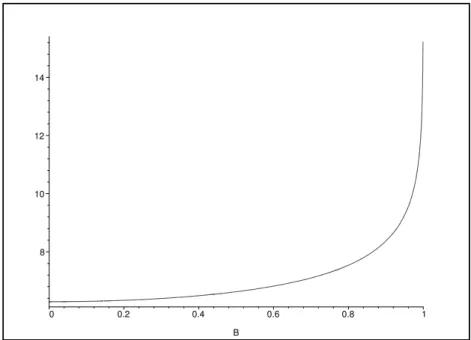
Example 1. ([BCS2000]) Consider a Randers- Minkowski norm of Nu-mata’s type
F(y1, y2) =p(y1)2+ (y2)2+By1
onR2, where B∈[0,1) is a constant parameter.
8 10 12 14
0 0.2 0.4 0.6 0.8 1
B
Figure 1. The variation of Riemannian length of the indicatrix for the metric given in Example 1.
Using polar coordinates
y1=rcosϕ, y2=rsinϕ,
the polar equation of the indicatrix is
r= 1
1 +Bcosϕ,
and the indicatrix length is given by the elliptic integral
(3.5) L= √ 4 1 +B
Z π 2
0
dµ
p
1−k2sin2µ,
whereϕ= 2µ, andk:= s
2B
1 +B.
We remark that for B ≡ 0, i.e. an Euclidean norm, one obtains L = 2π, as expected. The result of numerical estimation of the integral in (3.5) gives the graph in Figure 1.
One can see that unlike the Euclidean case, L increases to infinity when B
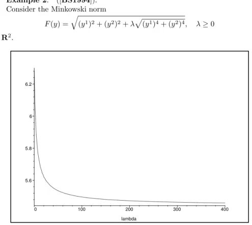
Example 2: ([BS1994]). Consider the Minkowski norm
F(y) = q
(y1)2+ (y2)2+λp(y1)4+ (y2)4, λ≥0
inR2.
5.6 5.8 6 6.2
0 100 200 300 400
lambda
Figure 2. The variation of Riemannian length of the indicatrix for the metric given in Example 2.
With the substitutionu:= y
2
y1 one obtains the indicatrix length
L= 8 Z 1
0
s
1 +λ (1 +u 2)3
(1 +u4)3/2+λ 2 3u
2
1 +u4
1 +u2+λ√1 +u4 du.
The numerical integration results are presented in Figure 2.
In this caseLdecreases from 2πto √3π asλ increases from 0 to∞. Indeed, one can see that
lim
λ→∞L=
√ 3π.
4. Finsler surfaces
This section follows the exposition in [BCS2000].
Let us consider, in the following, Finsler metrics defined on an orientable surface
M. Recall that aFinsler surface is the pair (M, F) where F : T M →[0,∞) is C∞ on T Mg := T M\{0} and whose restriction to each tangent plane T
xM is a
Minkowski norm.
For eachx∈Mthe quadratic formds2:=g
ij(x, y)dyi⊗dyjgives a Riemannian
functionFwe define theindicatrix bundle(orunit sphere bundle)IM :=∪x∈MIxM,
whereIxM :={y∈TxM :F(x, y) = 1}. Topologically,IxM is diffeomorphic with
the Euclidean unit sphereS2inR3. Moreover, the aboveds2induces a Riemannian
metrichx on eachIxM.
On the other hand, letSM :=T M/∼be the projective sphere bundle, where the equivalence relation “∼” is given byy∼y′ if and only if there existsλ >0 such
that y=λy′. The natural projectionπ:SM →M pulls back the tangent bundle
T M to a 2-dimensional vector bundleπ∗T M over the 3-dimensional manifoldSM.
Local coordinatesx1,x2 onM induce global coordinatesy1,y2on each fiberT
xM
by y = yi ∂
∂xi. Therefore (x
i, yi) is a coordinate system on SM (yi regarded as
homogeneous coordinates).
It is known ([BS1994]) that for each x∈ M, the canonical map i : IxM →
SxM, y7→[y] is a diffeomorphism, andi: (IxM, hx)→(SxM,g˙x) is a
Riemann-ian isometry, where ˙gxis the induced Riemannian metric on each projective sphere
SxM.
Let us also remark that since the Finslerian fundamental tensor gij(x, y) is
invariant under the rescalingy7→λy,λ >0, the inner products in the fibersTxM
are actually identical. This redundancy is removed by working with the pull-back bundleπ∗T M overSM.
Using the global sectionl:= y
i
F(y)
∂ ∂xi ofπ
∗T M, one can construct a positively
oriented g-orthonormal frame {e1, e2} for π∗T M, where g =gij(x, y)dxi⊗dxj is
the induced Riemannian metric on the fibers ofπ∗T M.
Namely,
e1:=
1 √g
∂F
∂y2 ∂ ∂x1−
∂F ∂y1
∂ ∂x2
=m1 ∂ ∂x1+m
2 ∂ ∂x2 ,
e2:= y1
F ∂ ∂x1+
y2 F
∂ ∂x2=l
1 ∂ ∂x1+l
2 ∂ ∂x2.
(4.1)
The frame {e1, e2} is a globally defined g-orthonormal frame field for π∗T M
called theBerwald frame. There are authors who consider the frame (l,−m) as the Berwald frame [M1986].
The corresponding dual coframe is
ω1= √g
F (y 2dx1
−y1dx2) =m1dx1+m2dx2
ω2= ∂F
∂y1dx 1+ ∂F
∂y2dx 2=l
1dx1+l2dx2.
(4.2)
The sphere bundle SM is a three dimensional Riemannian manifold with the Sasaki (type) metric
(4.3) ω1⊗ω1+ω2⊗ω2+ω3⊗ω3,
where
(4.4) ω3:= √g
F
y2δy 1
F −y 1δy
2
F
=m1
δy1 F +m2
Here, δ
δxi, F
∂ ∂yi
is a local adapted basis forT(T Mg), where
(4.5) δ
δxi:=
∂ ∂xi−N
j i
∂ ∂yj,
with the dual coframe{dxi,δy i
F}, where
(4.6) δyi:=dyi+Njidxj.
TheNi
j are the local coefficients of the Finslerian nonlinear connection (for details
see [BCS2000], [M1986]).
Remark 4.1. Remark that the above basis components F ∂ ∂yi, or
δyi
F are
”adjusted” such that they become an 0-homogeneous vector field, and a zero ho-mogeneous 1-form, respectively. In other words, the adapted basis components are invariant under the action ofy7→λy, for anyλ >0.
The globally defined orthonormal coframe{ω1, ω2, ω3} onSM has the dual
ˆ
e1=
1 √g
∂F
∂y2 δ δx1−
∂F ∂y1
δ δx2
=m1 δ δx1+m
2 δ δx2
ˆ
e2= y1
F δ δx1+
y2 F
δ δx2=l
1 δ δx1+l
2 δ δx2
ˆ
e3= F
√g ∂F
∂y2 ∂ ∂y1−
∂F ∂y1 ∂ ∂y2 =F
m1 ∂ ∂y1+m
2 ∂ ∂y2
.
(4.7)
Remark 4.2. (1) (dF)(ˆe1) = (dF)(ˆe2) = (dF)(ˆe3) = 0
Indeed, from δF
δxi = 0 it follows dF =
δF δxidx
i + ∂F
∂yiδy
i = ∂F
∂yiδy i.
Applying now this to ˆe1,ˆe2,ˆe3the result follows immediately.
(2) The vector ˆe3is tangent to each indicatrix.
(3) Using the indicatrix arc length formds= √g
F (y
1dy2−y2dy1) one sees that
ds(ˆe3) =−1, i.e. ˆe3 points opposite to the direction indicated as positive
byds.
Remark 4.3. Remark that the orthonormal coframe{ω1, ω2, ω3}onSM can
be completed to a g- orthonormal coframe {ω1, ω2, ω3, ω4} on the 4-dimensional
manifoldT M, where
ω4=d(logF) =l
i
δyi
F
(see [M1986] or [BCS2000] for details.)
Remark 4.4. Recall that on a Riemann-Finsler manifold, one have to deal with two kinds of metrics. This is easy to understand through a comparison with the Riemannian case.
(1) The Riemannian case. On a Riemannian manifold (M, g) the metric
is a specific inner product in each tangent spaceTxM viewed as a vector
space. Moreover,
(4.9) ˆg=gij(x)dyi⊗dyj
is an isotropic and constant Riemannian metric onTxM viewed as a
dif-ferentiable manifold.
(2) The Riemann-Finslerian case. On a Riemann-Finsler manifold (M, F) the metric
(4.10) g=gij(x, y)dxi⊗dxj
is a family of inner products in each tangent spaceTxM viewed as a vector
space, parametrized by raysty, (t >0) which emanate from origin. This is actually a Riemannian metric onπ∗T M. Moreover,
(4.11) ˆg=gij(x, y)dyi⊗dyj
is a non-isotropic Riemannian metric on TxM viewed as a differentiable
manifold, and which is invariant along each ray and possibly singular at the origin.
5. The Chern connection on Finslerian surfaces
This section summarizes some exposition in [BCS2000].
The vector bundleπ∗T Mhas a torsion-free and almostg-compatible connection
D:C∞(T SM)⊗C∞(π∗T M)→C∞(π∗T M), where
(5.1) DXˆZ :={Xˆ(zi) +zjωji( ˆX)}ei,
where ˆX is a vector field onSM,Z :=zie
i is a section ofπ∗T M, and{ei} is the
g-orthonormal frame field onπ∗T M.
Indeed, there is a unique set of connection 1-forms{ω i
j}onSM such that
dxj∧ωji= 0
(5.2)
dgij−gkjωik−gikωjk= 2Aijk
δyk
F , i, j, k∈ {1,2},
(5.3)
where δyk is given in (4.6), and A
ijk is the Cartan tensor of a Finsler metric
given by
(5.4) Aijk(x, y) =
F(x, y) 4
∂3F2(x, y) ∂yi∂yj∂yk.
The connection forms{ωij}define the well-knownChern connectionof the
Finsler manifold (M, F).
Remark 5.1. The torsion freeness condition (5.2) is equivalent to
(5.5) ω i
j = Γijkdxk
together with
(5.6) Γijk= Γikj,
where
(5.7) Γijk=
1 2g
is δgjs
δxk +
δgks
δxj −
δgjk
δxs
are the local coefficients of the Chern connection, and δ
Remark 5.2. A straightforward computation shows that the structure equa-tions (5.2), (5.3) of the Chern connection can be written also as
dωj=ωk∧ωkj
(5.8)
ωij+ωji=−2Aijkω2+k, i, j, k∈ {1,2},
(5.9)
where{ω1, ω2, ω3}is theg-orthonormal coframe on SM.
The following lemma provides a very useful formula for computations.
Lemma 5.1. With the above notations one has
(5.10) ∂gij
∂xk =gsjΓ s
ik+gsiΓsjk+ 2AijsN s k
F .
Indeed, by plugging (5.5) and (4.6) into the structure equation (5.3) one obtains (5.10).
The connection matrix (ω i
j ) of the Chern connection for Finsler surfaces with
respect to theg-orthonormal frame{e1, e2}ofπ∗T M is given by
(5.11)
ω11 ω12 ω21 ω22
=
−Iω3 −ω3
ω3 0
where I := A111 = A(e1, e1, e1) is the Cartan scalar for Finsler surfaces (for
details see [BCS2000]). Remark thatI= 0 is equivalent to the Finsler structure to be Riemannian.
We remark that if the Chern connection wereg-compatible, then the connection matrix (5.11) would have been skew-symmetric. It is known ([M1986]) that on a Finsler manifold there is no connection which possesses both torsion-freeness and
g-compatibility, except the case when the Finsler structure is actually Riemannian. One has to drop the torsion-freeness or the g-compatibility in order to work with Finsler metrics that are not Riemannian.
Cartan connection (see [M1986] for definition and details), for example, it is
g-compatible, but has some surviving torsion. On the other hand, the Chern con-nection used in the present paper claims for torsion-freeness but it can afford only almost g-compatibility (see (5.2) and (5.3)). In the case of the Chern connection, the connection matrix (5.11) is only “almost” skew-symmetric.
A regular piecewiseC∞ curveσ: [0, r]→M with velocity vectorT is called a
Finslerian geodesicif it satisfies the geodesic equation
(5.12) DT T
F(T)
= 0.
Remark 5.3. Observe that in natural coordinates one has
(5.13) ω12=
√g
F
y1δy 2
F −y 2δy
1
F
.
By taking the exterior derivatives and using torsion-free condition (5.2) one obtains thestructure equationsof a Finsler surface
dω1=−Iω1∧ω3+ω2∧ω3
dω2=−ω1∧ω3
dω3=Kω1∧ω2−Jω1∧ω3.
Remark 5.4. (1) For comparison, recall the structure equations of a Rie-mannian surface. They are obtained from (5.14) by settingI=J = 0. (2) The scalarK is called theGauss curvatureof a Finsler surface. In the
case whenF is Riemannian, Kcoincides with the usual Gauss curvature of a Riemannian surface.
Differentiating again (5.14) one obtains theBianchi identities
J =I2=
1
F
y1 δI δx1+y
2 δI δx2
K3+KI+J2= 0.
(5.15)
Here indices indicate directional derivatives along ˆe1, ˆe2, ˆe3, respectively. For
exampledK =K1ω1+K2ω2+K3ω3. The scalarsK1, K2, K3 are the directional
derivatives ofK.
Nevertheless, observe that the scalars I =I(x, y), J = J(x, y), K =K(x, y) and their derivatives lives onSM, not on M as in the Riemannian case!
More generally, given any functionf :SM → R, one can write its differential in the form
df=f1ω1+f2ω2+f3ω3.
Taking one more exterior differentiation of this formula, one obtains the fol-lowingRicci identities:
f21−f12 = −Kf3
(5.16)
f32−f23 = −f1
(5.17)
f31−f13 = If1+f2+Jf3.
(5.18)
The curvature 2-form of the Chern connection
(5.19) Ωi
j :=dωji−ωjk∧ωki
can be written by means of theg-orthogonal coframe as
(5.20) Ωji=
1 2R
i
j klωk∧ωl+Pj kli ωk∧ω2+l, i, j, k, l∈ {1,2}.
Indeed, let us remark first that (5.19) expands as follows
(5.21) Ωi j =
1 2R
i
j klωk∧ωl+Pj kli ωk∧ωl+n+
1 2Q
i
j klωk+n∧ωl+n,
where the coefficients R, P, Q are written in the cobasis ωi, andn = 2. The 1 2
coefficient appears because of the skew-symmetry ofR andQ, in other words, we have
(5.22) Rj kli =−Rj lki , Qj kli =−Qj lki .
Next, taking the exterior derivative of the torsion freeness condition (5.8) it follows
Ωkj∧ωk= 0,
and using this, (5.21) implies
(5.23) 0 = 1 2R
i
j klωk∧ωl∧ωj+Pj kli ωk∧ωl+n∧ωj+
1 2Q
i
It follows that all three coefficients in the right member of this equality have to vanish identically. Therefore, the symmetric part ofR and the skew-symmetric parts ofP andQhas to vanish, respectively, i.e.
Rj kli +Rk lji +Rl jki = 0,
Pj kli −Pk jli = 0, Qj kli −Qj lki = 0.
(5.24)
Now, from (5.22) and (5.24) it follows thatQi
j kl has to vanish, and therefore
(5.21) implies (5.20).
Moreover, this simplifies to
(5.25) Ω12=dω12=R1 122 ω1∧ω2+P2111ω1∧ω12.
Indeed, for a Finsler surface, from (5.11) follows the following important rela-tion
(5.26) Ωji=dωji,
i.e. the curvature form is an exact form, and therefore a closed one. Even though this formula is familiar in the Riemannian case, in the Finslerian setting it is a peculiarity of Finsler surfaces.
We rewrite (5.20) as
(5.27) Ωji=Rji12ω1∧ω2+Pj ki 1ωk∧ω3+Pji12ωk∧ω4
using the coframe{ω1,ω2,ω3,ω4}onT M.
Remark now that from the 0-homogeneity ofP it follows
(5.28) P i
j 12= 0
in theg-orthonormal coframe. Therefore, we obtain (5.29) Ωi
j =Rji12ω1∧ω2+Pj ki 1ωk∧ω3.
In the casei= 2,j= 1 we obtain
(5.30) Ω12=R1 122 ω1∧ω2+P1 112 ω1∧ω2+P1 212 ω2∧ω3.
Due to the properties of the tensorP, we have
P1 212 =P2 112 =P2211= 0
P1 112 =P1211=−P2111.
(5.31)
Let us remark that in the natural frame, the tensorP is not skew-symmetric in its first and second indices. However, the above formula is written in theg-orthonormal frame, and in this settingP becomes skew-symmetric in first and second indices if they contain an index equal to 2. The reason is that an index equal to 2 means contraction withli.
Using now (5.11) and (5.30) we obtain (5.25). Moreover, from (5.11) and (5.25) we obtain
(5.32) dω3=−R1 122 ω1∧ω2+P2111ω1∧ω3
and comparing this with (5.14) it follows
(5.33) K=R2112=−R1212, J=−P2111.
In the casei= 1,j= 1, (5.29) implies
On the other hand, from (5.11) and (5.14) we have
dω11=d(−Iω3) =−dI∧ω3−Idω3
=−(I1ω1+I2ω2+I3ω3)∧ω3−Idω3
= (Iω1+Iω2)∧ω3−I(Kω1∧ω2−Jω1∧ω3)
=−IKω1∧ω2−(I1−IJ)ω1∧ω3−I2ω2∧ω3.
(5.35)
It follows,
(5.36) R1112=−IK, P1111=IJ−I1.
Remark 5.5. The Gauss curvature K =R2112 is an important geometrical
quantity because its sign decides whether geodesic rays emanating from a common pointx∈M are going to focus or diverge (see [BCS2000]).
The Gauss curvature is the particularization to the case n = 2 of the flag curvature of an arbitrary dimension Finsler manifold. Indeed, one constructs a flag (x, y, V) atx∈M using
• a base pointx∈M, • a flag poley∈T]xM,
• an edgeV ∈TxM which is transversal to the flag pole.
Then
K(x, y, V) = gy(R(V, y)y, V)
gy(y, y)gy(V, V)−[gy(y, V)]2
= V
i(yjR
jiklyl)Vk
gy(y, y)gy(V, V)−[gy(y, V)]2
is called theflag curvatureof (M, F) and it is the Finslerian analog of the sectional curvature of a Riemannian manifold.
In arbitrary dimension, a Finsler metric F is said to be of scalar curvature ifK(x, y, V) does not depend onV. This can be rewritten as
Rik=K(x, y)(gik−lilk),
whereRik=ljRjiklll.
IfK=K(x, y, V) is a constant, thenF is said to be ofconstant flag curva-ture.
There is an essential difference between the Gauss curvature on Riemannian and Finslerian surfaces. If base pointxand the flag poleyare chosen, the tangent planeTxM is actually spanned byy and V, i.e. every Finsler surface is ofscalar
curvature K(x, y). By contrast, when the surface is Riemannian the scalar cur-vature K(x, y) reduces to the Riemannian Gauss curvature K(x), which does not depend ony.
There is another important difference between curvatures in Riemannian and Finslerian setting.
In Riemannian geometry the sectional curvature completely determine the cur-vature tensor (see for example [L1997] or another standard textbook of Riemannian geometry). This is not the case anymore for a Finsler manifold (arbitrary dimen-sion). The curvature form of the Chern connection Ωi
j contains two curvature
tensors: the so called (hh)-curvature tensor Rjikl and the (hv)-curvature tensor
of a Finsler manifold, is used for constructing the flag curvature and Jacobi equations.
6. Berwald and Landsberg surfaces
A Finsler surface is said to be ofLandsberg type ifJ = 0, or equivalently,
I2 = 0. Both Riemannian surfaces and (locally) Minkowski surfaces belong here.
Recall that a Finsler manifold (M, F) is calledlocally Minkowskiif there exists certain privileged local coordinates (xi) onM which, together with the coordinates
onT M induced byy=yi ∂
∂xi, makeF dependent only ony and notx([M1986],
[BCS2000]). Minkowski planes are always locally Minkowskian.
A stronger condition on a Finsler surface is that the Chern connection local coefficients depend only onx, i.e. Γi
jk(x, y) = Γijk(x). These Finsler surfaces are
said to be ofBerwald type.
The geometrical meaning of these special Finsler spaces can be described by means ofparallel translation.
Let us consider an arbitrary curveσ: [a, b]→M with velocity vector T(t) =
˙
σ(t), and an arbitrary vector fieldW(t) =Wi(t) ∂
∂xi|σ(t) alongσ.
Thelinear covariant derivative ofW alongσis defined by
(6.1) DTW := hdWi
dt +W
jTkΓi
jk(σ(t), T(t)) i ∂
∂xi|σ(t),
where Γi
jkare the coefficients of the Chern connection.
The vector fieldW(t) is said to belinearly parallel alongσ(t) ifDTW = 0.
Remark 6.1. Remark that in this case the Chern connection coefficients Γi jk
are evaluated alongσ, i.e. at the points (σ(t), T(t))∈Tσ(t)M. In other wordsthe
linear covariant derivative DTW is with reference vector T.
Remark also that if one deals with Berwald spaces, then the Chern connection coefficients satisfy Γi
jk(x, y) = Γijk(x), therefore the reference vector is irrelevant in
this case.
Remark 6.2. Recall that from the torsion-freeness and almost compatibility conditions of the Chern connection (5.2), (5.3) it follows
(6.2) d
dt
h
gT(U, V) i
=gT(DTU, V) +gT(U, DTV) + 2A(U, V, DTT),
for any two vector fieldsU, V alongσ.
Moreover, if one of the following three conditions holds (1) U orV is proportional toT,
(2) σis geodesic, (3) Avanishes alongσ, then
(6.3) d
dt
h
gT(U, V) i
=gT(DTU, V) +gT(U, DTV),
Let us consider now the case when the curveσ : [a, b]→M is a geodesic of the Finsler space (M, F). Thelinear parallel translationalongσ(t) is given by the map
(6.4) Pσ:Tσ(a)M →Tσ(b)M, Pσ(v) =w,
whereV(t) is a linearly parallel vector field alongσwithV(a) =v, V(b) =w. An immediate property of the linear parallel transport on Finsler manifolds follows ([CS2005]).
Lemma 6.1. Let (M, F)be a Finsler manifold,σ: [a, b]→M a geodesic ofF
with velocity vector T(t) = dσ
dt, and U(t), V(t) linearly parallel vector fields along σ. Then we have
(6.5) gT(t)
U(t), V(t)= 0.
Proof. Sinceσis geodesic, andU, V are two parallel vector fields alongσ, using Remark 6.2 it follows
d dt
h
gT(U, V) i
=gT(DTU, V) +gT(U, DTV) = 0.
ThereforegT(U, V) is constant alongσ.
Q.E.D. Letσ: [a, b]→M be again an arbitraryC∞piecewise curve onM with velocity
vectorT(t), and letW(t) be an arbitrary vector field alongσ.
Another way of defining the covariant derivative ofW is with reference vector
W. Indeed, thenonlinear covariant derivative ofW alongσis defined by
(6.6) D(TW)W :=hdW
i
dt +W
jTkΓi
jk(σ(t), W(t)) i ∂
∂xi
|σ(t),
where Γi
jkare the coefficients of the Chern connection. The top letter indicates the
reference vector. If it is absent it means that the reference vector isT. The vector fieldW(t) is said to benonlinearly parallelalongσ(t) ifDW
T W =
0.
Using this covariant derivative one can define another kind of parallel transla-tion of W alongσ. The nonlinear parallel translation along σ(t) is given by the map
(6.7) Pσn:Tσ(a)M →Tσ(b)M, Pσ(v) =w,
whereV(t) is a nonlinearly parallel vector field alongσwith V(a) =v, V(b) =w. The top letter n means “nonlinear”. If it is missing, then it means the linear parallel translation. This is the canonical parallel translation on a Finsler manifold.
Let us also remark that for a C∞ piecewise curve σ on a Finsler manifold
(M, F), the nonlinear parallel translation preserves the Finslerian norm, i.e. if
W(t) is nonlinearly parallel alongσ, thenF(σ(t), W(t)) =constant.
Lemma 6.2. ([I1978]) Let (M, F) be a Berwald manifold and σ: [a, b]→M
aC∞ curve on M with velocity vector fieldT(t) = dσ
dt. Then, the nonlinear parallel translationPn
σ :Tσ(a)M →Tσ(b)M is a linear isomorphism.
Proof. For a vector fieldV =Vi(t) ∂
∂xi that is nonlinearly parallel alongσ(t),
it follows
(6.8) hdV
i
dt +V
jTkΓi jk(σ)
i ∂
∂xi|σ(t)= 0,
where Γi
jk(σ, T) = Γijk(σ) are the coefficients of the Chern connection of the Berwald
manifold (M, F).
One can see that (6.8) is a linear ODE inV. Therefore it induces a linear map betweenTσ(a)M andTσ(b)M. The details follows immediately.
Q.E.D. Geometrically, Lemma 6.2 states that for a Berwald manifold, parallel transla-tion is an isometry of linear spaces.
Remark 6.3. In the proof of Lemma 6.2, the condition that the Finsler man-ifold (M, F) is a Berwald one is essential. Indeed, we used
(6.9) VjTkΓi
jk(σ, V) =VjTkΓijk(σ).
This relation is not true for other Finsler manifolds that are not of Berwald type.
Remark 6.4. In a Berwald space (arbitrary dimension) the Chern connection defines a linear connection directly on the underlying manifoldM.
Z. I. Szabo ([Sz1981]) proved that this linear connection is in fact the Levi– Civita connection of a (non-unique) Riemannian metric on M. In this way any Berwald space ismetrizableby such a Riemannian metric. Of course the Finsler metric and induced Riemannian metric onM have the same geodesics as curves on
M.
For a Landsberg surface, it is remarkable that the Gauss curvatureK at any pointy(t) of the indicatrixSxM is determined by the Cartan scalarIby
(6.10) K(t) =K(0)e−
hR
t 0I(τ)dτ
i
.
Indeed, from the Bianchi identities (5.15) on a Landsberg surface, i.e. whenJ = 0, one obtains the following ODE:
˙
K(t) +I(t)K(t) = 0.
Taking into account thatI(t) is continuous, the result follows directly by inte-gration ([BCS2000]).
Obviously, any Berwald space (arbitrary dimension) is a Landsberg space. Even though there are many examples of Berwald spaces, unfortunately concrete example of Landsberg spaces that are not Berwald are not studied yet enough. Especially the construction of such examples in the two dimensional case remains to be considered in the future. See Asanov’s recent results [A2006].
Theorem 6.1. Rigidity theorem for Berwald surfaces
Let(M, F)be a connected Berwald surface for which the Finsler structureF is smooth and strongly convex on all of T Mg.
(1) If K≡0, thenF is locally Minkowski everywhere.
(2) If K6≡0, thenF is Riemannian everywhere.
Proof. We give here the idea of the proof.
If on a surfaceK= 0, then (5.33), (5.36) implyR i j kl= 0.
On the other hand, the surface being Berwald it follows that the Chern con-nection coefficients depend on the position only, in other words Γi
jl(x, y) = Γijl(x),
therefore these coefficients determine a torsion free linear connectionDonM hav-ing the Christel coefficients precisely Γi
jl(x). It follows immediately that D must
be flat on M. Therefore there is a preferential coordinate chartx = (xi) on M
where Γi
jl(x) = 0, or equivalently,
∂gij
∂xk = 0. This is of course equivalent with
F(x, y) =F(y), i.e. F is locally Minkowski.
Conversely, if one assumes now that K 6≡ 0, then there exists an indicatrix
SpM, at a certain p ∈ M, such that K 6= 0 at some point of it, and therefore
nonzero at all points of thisSpM (because of (6.10)).
On a Berwald surface, the main scalar I is horizontally constant ([M1986], [BCS2000]), i.e. I1 =I2 = 0, where the subscripts means directional derivatives
with respect to the vectors of the g-orthonormal frame onSM.
Ricci identity (5.16) written for the Cartan scalarIon a Berwald surface implies
KI3 = 0, in other words onSpM we have KI˙= 0, and therefore I =constant on
thisSpM.
Taking into account the fact that the average value of the Cartan scalarIover the indicatrix TpM is zero ([BCS2000]), i.e. R0LI(t)dt = 0, one sees that this
constant has to be in fact zero. Therefore, F(p,y˜) has to be Riemannian for any ˜
y∈SpM.
On the other hand, recall from Lemma 6.2 that on a connected Berwald surface the Minkowski plane (TxM, F(x,·)) is linearly isometric to (TpM, F(p,·)) for any
x∈M.
SinceM is connected there exists a smooth pathσfrom xtop. If we denote by (x, y) and (p,y˜) the corresponding points in T M, respectively, and taking into account that ˜y is related toy by a linear transformation depending onxandσ, it follows thatF(x, y) is equal toF(p,y˜) and thereforeF is Riemannian everywhere. Q.E.D. The geometrical meaning of a Landsberg space is that the induced Riemann-ian tangent spaces (T]xM , gx) are isometric to each other by nonlinear parallel
translations.
Indeed, one has:
Lemma 6.3. ([I1978]) Let(M, F)be a Landsberg manifold, and letσ: [a, b]→
M, σ(a) =p∈M,σ(b) =q∈M, be a piecewise C∞ curve. Then, the nonlinear
parallel translation
(6.11) Pσn : (T]pM , gp)→(T]qM , gq)
For a proof see the paper [I1978].
On Landsberg surfaces, the following interesting properties hold.
Theorem 6.2. ([BS1994])
The indicatrix length of a Landsberg surface is constant.
Let us consider the Riemannian length of the indicatrix
Sx:={y∈TxM, F(x, y) = 1, x∈M}.
Recall from§2 that the indicatrix length is computed by integrating the Lands-berg angle.
Therefore, we have
(6.12) L(x) = Z
S1
the puredy part ofω12.
Some computations lead to the following lemma.
Lemma 6.4. ([BCS2000]) The Riemannian length of the indicatrix satisfies
(6.13) ∂L
∂xi= (−1) i
Z
S1
J(l3−i√g)dθ,
wherei∈ {1,2},dθis the 1-form given in (3.3),g is the determinant of the matrix gij, andJ is the scalar in (5.14).
Therefore the constantly of indicatrix length follows. However, typically this is NOT 2πas already shown in§2.
7. Curves on a Finsler surface
Let us consider the unit speed curveγ: [a, b]→M on a Finsler surface (M, F), given byxi=xi(t),T(t) = ˙γ(t),F(γ(t), T(t)) = 1, for anyt∈[a, b].
Using some ideas from [Sh2001], we are going to construct a Finslerian unit normal vector field N of γ such that the pair {T(t), N(t)} is an oriented gN
-orthogonal basis in the fiber ofπ∗T M over the point (γ(t), N(t)).
Proposition 7.1. For each fixed point x(t), t ∈ [a, b], on the curve γ, there exists a Finslerian unit length vector field N(t)∈T^x(t)M such that
(7.1) gN(t)(N(t), T(t)) = 0.
Proof. For eachx=x(t)∈M fixed, let us regardT]xM as a Minkowski plane
with the Minkowski normF(x, y) =F(y) induced by the Finslerian structureF of
M.
For the sake of simplicity we omit writing the dependency on the parametert
of the curve. All the vectors are assumed to be taken along the curveγ.
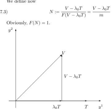
First of all, we are going to construct the vector N. Consider an arbitrary vectorV in the planeTxM, other thanT. Then the function
f :R→[0,∞), f(λ) :=F(V −λT)
attains its minimum for a unique valueλ0, i.e.
(7.2) min
λ F(V −λT) =F(V −λ0T) =m.
We define now
(7.3) N:= V −λ0T
F(V −λ0T)
= V −λ0T
m .
Obviously,F(N) = 1.
✲ ✻
✒
✲ ✲
✻
y1 y2
T λ0T
V
V −λ0T
Figure 3. The construction of the normal vector field.
Next, we are going to show that thisN is independent on the choice ofV. Let us consider another arbitrary vectorVe ∈TxM in the same upper half plane
(determined by the direction of the vectorT) asV. This vector can be written as a linear combination ofV andT, for example
(7.4) Ve =µ1V +µ2T, µ1>0.
Consider now the function
g:R→[0,∞), g(λe) :=F(Ve −eλT)
that attains its minimum for a unique valueλe0, i.e.
min
e
λ
F(Ve −λTe ) =F(Ve −eλ0T) =m.e
We can write now
e
m= min
e
λ
F(Ve −eλT) = min
e
λ
F(µ1V +µ2T−eλT)
=µ1min e
λ
F V −eλ−µµ2
1
T=µ1m.
(7.5)
SinceF(V −λT) attains its minimum atλ0(see (7.2)), it follows
(7.6) λ0=
e
λ0−µ2 µ1
.
Therefore, starting withVe we can construct the normal vector
(7.7) Ne :=Ve −eλ0T e
Using now (7.4), (7.5) and (7.6) in (7.7), a simple calculation shows thatNe=N, thereforeN does not depend on the choice of the directionV.
Finally, we are going to prove that thisN isgN orthogonal toT. Recall that
from the homogeneity condition ofF it follows
(7.8) gij(y)yi=
1 2
∂F2(y) ∂yj .
Indeed,F2is a 2-positive homogeneous function iny, therefore the Euler
the-orem for homogeneous functions gives ∂F
2(y)
∂yi ·y
i = 2F2(y). Taking now the
derivative of this relation with respect toyj, the relation (7.8) follows immediately. For anyV In the fiber ofπ∗T M over (γ(t), N(t)), relation (7.8) implies
(7.9) gN(N, W) =gij(N)NiWj=
1 2
∂F2(N) ∂yj W
j.
Consider now the function
(7.10) h:R→[0,∞), h(λ) := 1 2F
2(N+λT).
We have
h(λ) =1 2F
2V −λ0T
m +λT
= 1
2m2 F 2 V
−(λ0−mλ)T
≥ 2m12F 2(V
−λ0T) =
1 2m2 F
2(mN) = 1
2m2 m
2F2(N) = 1
2, for anyλ, where we have used (7.2).
In other words, the minimum ofhish(0) = 1 2. On the other hand,
h′(0) = 1 2
d dλ
F2(N+λT)|λ=0
= 1 2
∂F2
∂yj(N+λT)
d(N+λT)j
dλ
|λ=0.
Taking now into account the minimum of the functionhcomputed before, it follows
h′(0) =1 2
∂F2 ∂yj(N)T
j=g
N(N, T) = 0.
Q. E. D.
Remark 7.1. One can see that there exists exactly two normal vectors, one in the upper half plane determined by the direction ofT, and the other one in the opposite half plane. However, remark that these two normals are not parallel unless
F is absolute homogeneous.
We have therefore constructed a Finslerian unit normal vector fieldN =N(t) along the curveγ with the following properties
(1) N isgN-orthogonal toT,
We have to remark however, that in the fiber over (γ(t), N(t)) we haveF2(T)6= gN(T, T). We denote this quantity by σ2 := gN(T, T). Therefore, the frame {T(t), N(t)} is not a gN-orthonormal basis, but only a gN-orthogonal one. In
the particular case whenM is a Riemannian surface with the Riemannian metric
g, the pair{T(t), N(t)}is ag-orthonormal basis.
Next, we will define the geodesic curvature for the curveγon the Finsler surface (M, F).
Let us recall that ifM is a Riemannian surface with the Riemannian metricg, then
(7.11) K(t) :=DTT =
d2xi
dt2 +γ
i jk(x)
dxj
dt dxk
dt
∂ ∂xi|γ(t)
is called thegeodesic curvature vectorof the curveγ,
(7.12) k(t) :=g(K(t),K(t)) 1 2
is called thegeodesic curvature ofγ, and
(7.13) kN(t) :=g(K(t), N(t))
is called the signed curvature of γ. Here, D is the Levi-Civita connection of g
and γi
jk(x) the Christoffel coefficients ofD. Recall also that if γ is a geodesic of
the Riemannian metricg, thenK(t),k(t) andkN(t) all vanish. In other words the
geodesic curvature vector K(t) measures the failure of the curveγ from being a geodesic.
Now we return to the more general case of a Finsler surface. We would like to define a geodesic curvature vector and a geodesic curvature with similar prop-erties as in the Riemannian case. Keeping in mind the geometrical meaning these quantities should have, one might define
(7.14) K(T)(t) :=DT(T)T =
dTi
dt + Γ
i
jk(x, T)TjTk ∂
∂xi|γ(t)
and
(7.15) k(T)(t) :=g
T(K(T)(t),K(T)(t)) 1
2.
These quantities might be called thegeodesic curvature vector overT, and the geodesic curvature over T of the curveγ, respectively.
Remark two things about the quantities defined in (7.14), (7.15): (1) they are defined in the fiber of π∗T M over (γ(t), T(t)),
(2) ifγis a geodesic of the Finsler structure, in other words the tangent vector field is autoparallel alongγ, i.e. DT(T)T = 0, then bothK(T)(t) andk(T)(t)
vanish like in the Riemannian case (see [BCS2000] for more on Finslerian geodesics).
These definitions are used in [Sh2001].
We are led in this way to the following definitions. Let
(7.16) K(N)(t) :=D(N)
T N =
dNi
dt + Γ
i
jk(x, N)NjTk ∂
∂xi|γ(t)
and
(7.17) k(N)(t) :=gN(K(N)(t),K(N)(t)) 1
2
be thegeodesic curvature vector over N, and thegeodesic curvature over N of the curveγ, respectively.
We remark that the quantities defined in (7.16), (7.17)
(1) are defined in the fiber ofπ∗T M over (γ(t), N(t)),
(2) ifγ is a geodesic, i.e. D(TT)T = 0, thenK(N)(t) andk(N)(t) do not vanish
anymore as in the Riemannian case. Instead, ifγis a curve along whichN
is parallely displaced, i.e. D(TN)N = 0, then they will vanish. The reason
behind this strange fact is that in the Riemannian case along a geodesicγ
the conditionsDTT = 0 andDTN = 0 are equivalent, but for a Finslerian
surface,D(TT)T = 0 andD(TN)N= 0 are not.
Let us assume thatγis a smooth closed curve in the plane. Then we can regard
γ as the boundary of a bounded open set Ω⊂M. Recall that ifγ is parametrized so that T(t) is consistent with the induced orientation onγ =∂Ω in the sense of Stokes’ theorem, thenγis calledpositively oriented. Intuitively, this means that
γ is parametrized in the counterclockwise direction, or that Ω is always to the left ofγ([L1997]).
We can regard now{T(t), N(t)}as an orientedgN-orthogonal basis forTγ(t)M
for eacht. Ifγ is positively oriented as the boundary of Ω, this is equivalent toN
being the inward-pointing normal to∂Ω.
Using now (7.16) we define thesigned curvature over Nofγ by
(7.18) k(NN)(t) :=−gN(K(N)(t), T(t)),
whereT(t) is considered now as a vector field in the fiber ofπ∗T Mover (γ(t), N(t)).
Remark 7.2. If (M, F) is an absolute homogeneous Finsler metric, or a Berwald metric, then the sign of kN(N) is positive if γ is curving towards Ω, and
negative if it is curving away. This is the meaning of the word “signed” here. In the more general case of a Finsler metric (only positive homogeneous), the sign of kN(N) is positive ifγ is curving towards Ω, but it is difficult to predict how this changes ifγis curving away (see (7.16)).
We will see in the next section why we prefer our definitions (7.16), (7.17) to Shen’s definitions (7.14), (7.15).
Lemma 7.1. Let U(t)and V(t)be two vector fields along the curve γ. Then we have:
(7.19) d
dt gN(U, V) =gN(D (N)
T U, V) +gN(U, D(TN)V) + 2A(U, V, D
(N)
Proof. By straightforward computation and use of Lemma 5.1 we have:
d
dt gN(U, V) = d
dtgij(x, N)U
iVj+g
ij(x, N) dUi
dt V
j+UidV j
dt
=gsjΓsik+gsiΓsjk+ 2Aijs
Ns k
F
(x, N)TkUiVj
+ 2Aijk
F (x, N) dNk
dt U
iVj
+gij(x, N) dUi
dt V
j+UidVj
dt
,
(7.20)
where Ns
k(x, N) = NjΓsjk(x, N) is the nonlinear connection of F. Grouping now
these terms, and taking into account of (6.6), relation (7.19) follows easily.
Q. E. D.
Remark 7.3. If one of the following conditions holds (1)U or V is proportional toN,
(2)N is parallel transported alongγ, (3)A vanishes alongγ,
then,
(7.21) d
dtgN(U, V) =gN(D (N)
T U, V) +gN(U, DT(N)V).
One might remark also that Lemma 7.1. is in fact the “with reference vector
N” version of the Remark 6.2.
From Remark 7.3. it also follows that the signed curvature k(NN) ofγ defined
in (7.18) can be also written as
k(NN)(t) =gN(D(TN)T, N).
One can remark that in the Riemannian case this coincides with the usual signed curvature ofγdefined in (7.13).
Proposition 7.2. If γ is a smooth curve on the Finsler surface (M, F), then the following relations hold good
K(N)(t) = − σ21(t) k (N)
N (t)T(t),
(7.22)
k(N)(t) = 1
σ(t)|k
(N)
N (t)|,
(7.23)
whereσ2(t) =g
N(T, T), andK(N)(t),k(N)(t),kN(N)(t)are defined in (7.16), (7.17),
(7.18), respectively.
Proof. Using Remark 7.3., in the caseU =V =N, it followsgN(DT(N)N, N) =
0. In other words, the geodesic curvature tensorK(N)(t) =DT(N)NisgN-orthogonal
toN. This implies that there exists a smooth functionf such that
(7.24) K(N)(t) =DT(N)N =f(t)T(t),
whereT is the tangent vector toγ in the fiber ofπ∗T M over (γ, N).
We compute now
It follows
(7.25) kN(N)(t) =−f(t)σ2(t),
and therefore from (7.24), (7.25) we obtain (7.22). Next, we compute
(k(N)(t))2=gN(K(N)(t),K(N)(t)) =
1
σ4(t)(k (N)
N (t))2gN(T, T)
= 1
σ2(t)(k (N)
N (t))2,
and (7.23) follows immediately.
Q. E. D.
8. The Gauss-Bonnet Theorem for Finsler surfaces
The proof of the Gauss-Bonnet theorem for Finsler manifolds without bound-ary was given by D. Bao and S. S. Chern in [BC1996] using the transgression method. Using their method we will extend the result to Finsler surfaces with smooth boundary.
Let (M, F) a compact Finsler surface with smooth boundary∂M =γ: [a, b]7→
M, given by xi = xi(t). We assume γ to be unit speed, i.e. F(T) = 1, where
T = ˙γ(t).
For an arbitrary vector fieldV :M →T M,x7−→V(x)∈TxM, denote its zeros
byx1,· · ·, xk ∈M, and denote byiαthe index ofV atxα, for allα= 1,2,· · ·, k.
By removing from M the interiors of the geodesic circles Sε
α (centered at xα of
radius ε >0), one obtains the manifold with boundaryMε. Remark that in this
case, the boundary ofMεconsists of the boundaries of the geodesic circlesSαε and
the boundary ofM.
Assuming thatV has all zeros in M \∂M, it follows thatV has no zeros on
Mεand therefore we can normalize it obtaining in this way the application
(8.1) X = V
F(V):Mε→SM, x7→
V(x)
F(V(x)).
Using X we can lift Mε to SM constructing in this way the 2-dimensional
submanifoldX(Mε) ofSM.
Recall that on the 3-dimensional manifoldSMone has the exterior forms, Ω12
andω12, defined in (5.19) and (5.11), respectively.
Proposition 8.1. Let (M, F) be a compact oriented Landsberg surface with boundary ∂M. And let N : ∂M → SM be the inward pointing Finslerian unit normal on ∂M.
Then, we have
(8.2) 1
L
Z
M
K√g dx1∧dx2+ 1 L
Z
N(∂M) ω 2
1 =X(M),
where Lis the Riemannian length of the indicatrix, K andg the Gauss curvature and the determinant of the fundamental tensor gij of the Finsler metric,
The proof follows [BCS2000]. Indeed, remark first that we can extend the normal vector field N on γ to a vector field X on M with only finitely many zeros x1, x2, . . . xk ∈ M \∂M. By considering the lift X(Mε) constructed above
we integrate formula (5.25) over the two dimensional manifold X(Mε). Applying
Stokes’ theorem and taking the limitε→0, we obtain
(8.3) Z
M
X∗(R1212ω1∧ω2+P2111ω1∧ω12) =
k X
α=1
lim
ε→0
Z
X(Sε α)
ω12+
Z
N(∂M) ω12,
where the liftX(Sε
α) of each boundary cycle is traced out in the clockwise direction,
andN is the inward pointing normal to the boundary∂M.
From the degree theory (see for example [Mil1965]) it results that Z
X(Sε α)
ω12−→ −iα Z
SxαM
ω12
asε→0. Here the indicatrixSxαM is given in the counterclockwise orientation.
Recall now that
ω12=
√g
F
y1δy 2
F −y 2δy
1
F
,
whereδyi =dyi+Ni
jdxj. Taking the limit of the integralω12implies that actually
the dx terms do not contribute anymore because the metric radius continuously shrinks. It follows that
(8.4) lim
ε→0
Z
SxαM
ω12= lim
ε→0
Z
S1
√g
F2
y1dy2−y2dy1
=L(xα),
whereL(xα) is the Riemannian length of the indicatrix atxα∈M.
Let us consider now the case of Landsberg surfaces. There are three important results that make these surfaces special.
(1) On a Landsberg surface P2111 =−J = 0, therefore the integrand in the
left hand side of (8.3) reads now Ω12=dω12=R1212 ω1∧ω2. In natural
coordinates we have
Ω12=dω12=−K√g dx1∧dx2.
(2) Moreover, even though K=K(x, y) and√g=√g(x, y) are functions on
SM, their productK√g= (K√g)(x) lives onM. Indeed, taking exterior derivative ofdω12=−K√g dx1∧dx2 it follows
d(K√g)∧dx1∧dx2= 0,
or equivalently, ∂(K√g)
∂xi dx
i+∂(K √g)
∂yi dy i
∧dx1∧dx2= 0.
Taking into account the properties of exterior differentiald, it follows
∂(K√g)
∂yi = 0. This was remarked by S. S. Chern for the first time (see
[BC1996] for details).
Therefore, the first term in the left hand side of (8.3) simplifies to
(8.5)
Z
M−
(3) Finally, recall that on a Landsberg surface, the indicatrix lengthL(x) is a constant, but this constant typically is not equal to 2πas in Riemannian case. From (8.4) it follows that on a Landsberg surface we have
(8.6)
k X
α=1
lim
ε→0
Z
X(Sε α)
ω12=−
k X
i=1
iαL(xα) =−L k X
i=1
iα=−LX(M).
Using now (8.5) and (8.6) in (8.3) we obtain two of the three terms in (8.2).
We are going to deduce now the remainig term on the left hand side of (8.2). In order to do this, let us remark first that the normal N(t) introduced in Proposition 7.1. can be regarded as the mapping
(8.7) N :∂M =γ→SM γ(t)7→(γ(t), N(t)),
whereSM is the projective sphere ofF.
This gives the lift ˆγ=N(∂M) of the curveγ toSM given by
(8.8) γˆ: [0,1]→SM, γˆ(t) = (γ(t), N(t)).
Remark that ˆγ is different from the canonical lift (γ(t),γ˙(t)) of γ used in the monograph [BCS2000].
The tangent vector ˆT to ˆγ in a pointu= (γ(t), N(t))∈γˆ is given by
ˆ
T = d
dtˆγ= ˙γ
i(t) ∂
∂xi|(γ,N)+
dNi(t)
dt ∂ ∂yi|(γ,N)
= ˙γi(t) δ
δxi|(γ,N)+
hdNi(t)
dt +N
j(t) ˙γk(t)Γi jk(γ, N)
i
|(γ,N)
= ˙γi(t) δ
δxi|(γ,N)+ (D
(N)
T N) i ∂
∂yi|(γ,N),
(8.9)
where the functions Γi
jk are the local coefficients of the Chern connection, and
(DT(N)N)i are the components in the natural basis of the fiber of the covariant
derivative alongγ with reference vectorN defined in (6.6).
One can easily see that this ˆT gives the derivative map of the mapping N :
∂M →SM. Indeed, (8.7) implies
(8.10) N∗,γ(t):Tγ(t)∂M →T(γ(t),N(t))SM, N∗,γ(t)
d
dt|γ(t)
= ˆT(t),
where d
dt|γ(t)is the natural basis ofTγ(t)∂M.
Now we can prove the following important result.
Proposition 8.2. On the Finsler manifold (M, F) with the smooth boundary ∂M =γ: [a, b]→M we have
(8.11)
Z
N(∂M) ω12=
Z
γ
1
σ(t) k
(N)
N (t)dt,
whereN is the inward pointing normal onγ,ω 2
Proof.
Using (8.9) and (8.10) we compute
N∗(ω12) d
dt|γ(t)=ω 2 1 (N∗
d dt)
=ω12
h ˙
γi(t) δ
δxi|(γ,N)+ (D
(N)
T N) i ∂
∂yi|(γ,N) i
= ˙γi(t)ω12
δ
δxi|(γ,N)
+ (D(TN)N)iω12
∂
∂yi|(γ,N)
.
(8.12)
On the other hand, recall the local expression (5.13) of the connection formω 2 1 ,
and taking into account the duality of the natural basis {δxδi, F
∂
∂yi} and cobasis
{dxi,δy i
F } it follows that the first term in the last equality of (8.12) vanishes and
therefore we obtain
N∗(ω12) d
dt|γ(t)= (D (N)
T N) iω 2
1
∂
∂yi|(γ,N)
= (DT(N)N)1ω12
∂
∂y1|(γ,N)
+ (D(TN)N)2ω12
∂
∂y2|(γ,N)
=√g(γ, N)h−y2(DT(N)N)1+y1(D(TN)N)2i
|(γ,N)
=√g(γ, N)h−N2(DT(N)N)1+N1(D
(N)
T N)2 i
.
(8.13)
We used here implicitly thatF(γ, N) = 1.
We would like now to express this relation using the signed geodesic curvature
k(TN)defined in (7.18). In order to do this, remark that writing (7.21) forU =V =
N, and taking into accountF(N) = 1, it followsgN(D(TN)N, N) = 0. We write this
last relation and (7.18) in the components with respect of the natural basis of the fiber of π∗T M over (γ, N). We have
(DT(N)N)1(N1g11+N2g12) + (DT(N)N)2(N1g12+N2g22) = 0
(DT(N)N)1( ˙γ1g11+ ˙γ2g12) + (D(TN)N)
2( ˙γ1g
12+ ˙γ2g22) =−k(NN),
wheregij,i, j∈ {1,2}are the components of the Riemannian metricgN of the fiber
ofπ∗T M over the point (γ, N) with respect to the natural basis of the fiber.
This is a system of linear equations with the solution
(D(TN)N)1=−k(N)
N
N1g
12+N2g22 g(N2γ˙1−N1γ˙2)
(D(TN)N)2=k(NN) N 1g
11+N2g12 g(N2γ˙1−N1γ˙2).
(8.14)
Substituting now (8.14) in the last equality of (8.13) we have
N∗(ω12) d
dt|γ(t)=k (N)
N
N2(N1g
12+N2g22) +N1(N1g11+N2g12)
√g(N2γ˙1−N1γ˙2)
=k(NN)√ gN(N, N) g(N2γ˙1−N1γ˙2)=
k(NN)
√g(N2γ˙1−N1γ˙2).
On the other hand, we remark that
(8.16) √g(N2γ˙1−N1γ˙2) =√gdx1∧dx2(T, N) =√gθ¯ 1∧θ2(T, N),
whereθ1andθ2 are the dual 1-forms ofT andN, respectively, and ¯g is the
deter-minant of the Riemannian metric in the fiber ofπ∗T M over (γ, N) with respect to
thegN orthogonal basis {T, N}, i.e.
(8.17) ¯gij(γ, N) =
1 0 0 σ2
and therefore its determinant is ¯g=σ2.
It follows
(8.18) √g(N2γ˙1−N1γ˙2) =σ
and from here we obtain
(8.19) N∗(ω12) d dt|γ(t)=
kN(N) σ(t).
Finally, we have
(8.20)
Z
N(∂M) ω12=
Z
∂M
N∗(ω12) =
Z
γ
N∗(ω12) d
dt|γ(t)dt=
Z
γ
kN(N) σ(t)dt.
Q. E. D. From Propositions 8.1. and 8.2. we obtain the main result of this section.
Theorem 8.1. Gauss-Bonnet theorem for Landsberg surfaces with smooth boundary.
Let(M, F)be a compact, connected Landsberg surface with unit velocity smooth boundaryγ. Then
(8.21) 1
L
Z
M
K√g dx1∧dx2+ 1
L
Z
γ
1
σ(t) k
(N)
N (t)dt=X(M),
whereLis the Riemannian length of the indicatrix of(M, F),k(NN) the signed
cur-vature over N ofγ, the scalarσ=pgN(T, T), andX(M)the Euler characteristic
of M.
Remark 8.1. (1) On a Berwald surface without boundary an alternative Gauss-Bonnet formula can be given using the Riemannian metrizability of the Berwald surface ([BCS1996]). Indeed, let us denote by h the (non-unique) Riemannian metric onM having the Levi-Civita connection coefficients identical with the Chern connection coefficients of (M, F). Denote byhK its Riemannian Gauss curvature. Therefore the following
formula also holds:
(8.22)
Z
M
hK√hdx1
∧dx2= 2π· X(M).
(3) In the case of a Riemannian surface with smooth boundary, since the Rie-mannian metric has no directional dependence, and the indicatrix length of a Riemannian manifold is equal to 2π, Theorem 8.1 reduces to the usual Gauss-Bonnet theorem for Riemannian manifolds with smooth boundary [Spiv1979], [L1997].
Acknowledgments. The authors would like to express their gratitude to David Bao for his criticism and a very attentive check of the paper, and to Gheo-rghe Pitis for many useful discussions on the Gauss-Bonnet theorem in Riemannian geometry. We are also thankful to Katsuhiro Shiohama and Jin-ichi Itoh for bring-ing into our attention the importance of Gauss-Bonnet theorem for manifolds with boundary.
References
[A2006] Asanov, G.S., Finsleroid-Finsler space and Spray coefficients, arXiv:math.DG/0604526v1, 2006.
[BC1996] Bao, D., Chern, S.S., A Note on the Gauss-Bonnet Theorem for Finsler spaces, Annals of Math.,143(1996), 233–252.
[BCS1996] Bao, D., Chern, S.S., Shen, Z.,On the Gauss-Bonnet integrand for 4-dimensional Landsberg spaces, Contemp. Math,196(1996), 15–25.
[BCS2000] Bao, D., Chern, S.S., Shen, Z., An Introduction to Riemann Finsler Geometry, Springer, GTM 200, 2000.
[Errata] The errata of [BCS2000], the file can be downloaded from D. Bao’s site: http://math.uh.edu/˜bao/BCS-errata.pdf.
[BS1994] Bao, D., Shen, Z., On the volume of unit tangent spheres in a Finsler manifold, Results in Math.,26(1994), 1–17.
[CS2005] Chern, S.S., Shen, Z.,Riemann-Finsler Geometry, World Scientific Publishers, 2005. [I1978] Ichijyo, Y.,On special Finsler connections with vanishinghv-curvature tensor,
Ten-sor N.S.,32(1978), 146–155.
[L1997] Lee, J.M.,Riemannian manifolds: An Introduction to curvature, Springer, 1997. [M1986] Matsumoto, M.,Foundations of Finsler Geometry and Special Finsler Spaces,
Kai-seisha Press, Otsu, Japan, 1986.
[Mil1965] Milnor, J.,Topology from the differentiable viewpoint, University Press of Virginia, Charlotesville, 1965.
[R1959] Rund, H.,The Differential Geometry of Finsler Spaces, Springer-Verlag, 1959. [Sh2001] Shen, Z.,Lectures on Finsler Geometry, World Scientific, 2001.
[Sh2004] Shen, Z., Landsberg curvature, S-curvature and Riemann curvature, A Sampler of Riemann-Finsler Geometry, MSRI Publications,50(2004), 303–355.
[SST2003] Shiohama, K., Shioya, T., Tanaka, M.,The geometry of total curvature on complete open surfaces, Cambridge University Press, 2003.
[Spiv1979] Spivak, M.,A Comprehensive Introduction to Differential Geometry, Second Edition,
Vol. V, Publish or Perish, Inc., 1979.
[Sz1981] Szab´o, Z. I.,Positive definite Berwald spaces (Structure theorems on Berwald spaces), Tensor N.S.,35(1981), 25–39.
Hokkaido Tokai University, Sapporo, Japan E-mail: [email protected]