An empirical evaluation of outlier deletion methods for analogy-based cost estimation

全文

(1)An Empirical Evaluation of Outlier Deletion Methods for Analogy-Based Cost Estimation Masateru Tsunoda. Akito Monden. Nara Institute of Science and Technology Kansai Science City, 630-0192 Japan. Nara Institute of Science and Technology Kansai Science City, 630-0192 Japan. masate-t@is.naist.jp. akito-m@is.naist.jp. Takeshi Kakimoto. Ken-ichi Matsumoto. Kagawa National College of Technology 355 Chokushicho, Takamatsu-shi, Kagawa 761-8058 Japan. Nara Institute of Science and Technology Kansai Science City, 630-0192 Japan. kakimoto@t.kagawa-nct.ac.jp. matumoto@is.naist.jp. ABSTRACT Background: Any software project dataset sometimes includes outliers which affect the accuracy of effort estimation. Outlier deletion methods are often used to eliminate them. However, there are few case studies which apply outlier deletion methods to analogy-based estimation, so it is not clear which method is more suitable for analogy-based estimation. Aim: Clarifying the effects of existing outlier deletion methods (Cook’s distance based deletion, LTS based deletion, k-means based deletion, Mantel’s correlation based deletion, and EID based deletion) and our method for analogy-based estimation. Method: In the experiment, outlier deletion methods were applied to three kinds of datasets (the ISBSG, Kitchenham, and Desharnais datasets), and their estimation accuracy evaluated based on BRE (Balanced Relative Error). Our method eliminates outliers from the neighborhoods of a target project when the effort is extremely different from other neighborhoods. Results: Deletion methods which are designed to apply to analogy-based estimation (i.e. Mantel’s correlation based deletion, EID based deletion, and our method) showed stable performance. Especially, only our method showed over 10% improvement of the average BRE on two datasets. Conclusions: It is reasonable to apply deletion methods designed for analogy-based estimation, and more preferable to apply our method to analogybased estimation.. Categories and Subject Descriptors D.2.9 [Software Engineering]: Management – Cost estimation, K.6.1 [Computing Milieux]: Project and People Management – Staffing. Permission to make digital or hard copies of all or part of this work for personal or classroom use is granted without fee provided that copies are not made or distributed for profit or commercial advantage and that copies bear this notice and the full citation on the first page. To copy otherwise, or republish, to post on servers or to redistribute to lists, requires prior specific permission and/or a fee. PROMISE '11, September 20-21, 2011, Banff, Canada. Copyright 2011 ACM 978-1-4503-0709-3/11/09... $10.00.. General Terms Management, Measurement, Economics, Experimentation.. Keywords Case based reasoning, effort prediction, abnormal value, project management, productivity.. 1. INTRODUCTION To achieve success for a software development project, the development effort must be accurately estimated, so many quantitative estimation methods have been proposed [2][24][27]. Recently, analogy-based estimation [26] has gained attention, and many proposals and case studies have been reported [9][10][19][28][29]. Analogy-based estimation selects projects (neighborhood projects) which are similar to the estimated project from a past project dataset, and estimates effort based on the similar projects’ effort. One of the advantages of analogy-based estimation is that estimation results are comprehensible for estimators such as project managers [29], because they can confirm the neighborhood projects used for estimation. Although ordinary estimation models such as a linear regression model estimate various target projects’ effort using a model, analogy-based estimation does not make such a model, estimating effort only by neighborhood projects’ effort. So analogy-based estimation can reflect the individuality of each target project in the estimation. A past project dataset sometimes includes project data which should not be used for estimation [25]. For example, projects where an exceptional amount of rework occurred have a larger effort than other projects of the same scale (atypical cases). Additionally, when the effort was inaccurately collected or recorded, the recorded effort is different from the actual effort (noisy cases). Both atypical cases and noisy cases should be eliminated from the dataset before estimating effort, because their effort is quite different from projects whose features are similar to them, and that lessens estimation accuracy. However, to identify these projects is not easy because the internal details of each project are usually.

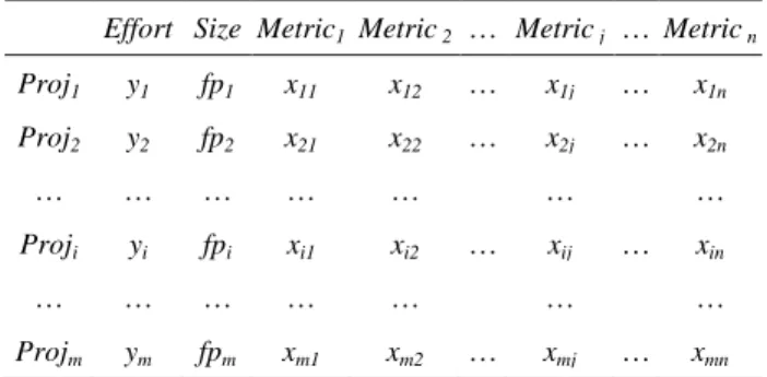
(2) not recorded in the dataset. Even if such details can be grasped, it is difficult to settle the elimination criteria (For example, it is difficult to settle the criterion for an abnormal amount of rework). Statistical outlier deletion methods are often used to eliminate such projects (That is, such projects are treated as outliers). Outlier deletion methods identify projects as outliers when the values of specific variables are extremely large or a combination of the values of variables (e.g. the combination of effort, system size, and team size) is fairly different from values for other projects, and remove the outliers from the dataset. Cook’s distance is widely used as an outlier deletion method when applying linear regression analysis. In addition to Cook’s distance, some outlier deletion methods for effort estimation [5][15][25] have been proposed. However, there are few case studies which apply outlier deletion methods to analogy-based estimation and compare their effects on analogy-based estimation. So, it is not clear which deletion method is more suitable for analogy-based estimation. In this research, we apply outlier deletion methods to analogybased estimation to compare their effects. Five types of outlier deletion methods (EID (Effort Inconsistency Degree) based deletion [15], Mantel’s correlation based deletion [9], Cook’s distance based deletion, k-means based deletion [25], and LTS (Least trimmed squares) based deletion [25]) were applied to the ISBSG [8], Kitchenham [14] and Desharnais datasets [7], with development effort estimated by analogy-based estimation. These datasets include data about many projects collected from software development companies, and are widely used in many researches. Additionally, considering the characteristics of analogy-based estimation, we applied our outlier deletion method and compared its effect with others. In analogy-based estimation, when the variance of the actual effort of neighborhood projects is large, the estimation accuracy becomes low [23]. Our method identifies a project as an outlier when the effort of the project is significantly higher or lower than other neighborhood projects, and excludes it from the computation of estimated effort. The actual effort of neighborhood projects is normalized by robust Z-score computation [22], and when the normalized value is larger than a threshold, the project is identified as an outlier. While existing deletion methods eliminate outliers from the entire dataset before estimation, our method eliminates outliers from neighborhood projects. Below, Section 2 explains analogy-based estimation. Section 3 explains outlier deletion methods, and Section 4 describes the experimental setting. Section 5 shows results of the experiment and discusses it, and Section 6 concludes the paper with a summary.. Table 1. Dataset used by analogy-based estimation Effort Size Metric1 Metric 2 … Metric j … Metric n Proj1. y1. fp1. x11. x12. …. x1j. …. x1n. Proj2. y2. fp2. x21. x22. …. x2j. …. x2n. …. …. …. …. …. Proji. yi. fpi. xi1. xi2. …. …. …. …. …. Projm. ym. fpm. xm1. xm2. … …. … …. xij …. …. xin …. xmj. …. xmn. without a stored software project dataset, analogy-based estimation cannot estimate without it. This is a weak point of analogybased estimation, but it can be overcome by using public datasets. Analogy-based estimation uses an m×n matrix as shown in Table 1. In the matrix, Proji is i-th project, Metricj is j-th variable, xij is a value of Metricj of Proji, fpi is the development size (e.g. function point) of Proji, and yi is the actual effort of Proji. We presume ˆ. Proja is the estimated project, and ya is the estimated value of ya. The analogy-based estimation procedure consists of the three steps described below. Step 1: Since each variable Metricj has a different range of values, this step normalizes the ranges from [0, 1]. The normalized value xíj, is calculated from the value of xij by:. xij . xij  min Mertic j . max Metric j   min Metric j . (1). In this equation, max(Metricj) and min(Metricj) denote the maximum and minimum value of Metricj respectively. Step 2: To find projects which are similar to the estimated project Proja (i.e. identifying the neighborhood projects), the distance between Proja and other projects Proji is calculated. Although various measures (e.g. a measure directly handling nominal variables) have been proposed [1], we applied the Euclidean distance measure because it is widely used [28]. In this measure, a short distance indicates that two projects are similar. The distance Dist(Proja, Proji) between Proja and Proji is calculated by: DistProja , Proji  .  x  m. h 1. ah.  xih h . 2. (2). ˆ. 2. ANALOGY-BASED ESTIMATION Analogy-based estimation originated with CBR (case based reasoning), which is studied in the artificial intelligence field. Shepperd et al. [26] applied CBR to software development effort estimation. CBR selects a case similar to a current issue from a set of accumulated past cases, and applies the solution of the case to the issue. CBR assumes that similar issues can be solved by a similar solution. Analogy-based estimation assumes that similar neighborhood projects (for example, with similar development size and programming languages) have similar effort, and estimates effort based on the neighborhood projects’ effort. Although ready-made estimation models such as COCOMO [2] can make estimates. Step 3: The estimated effort ya of project Proja is calculated from the actual effort yi of k neighborhood projects. While the average of the neighborhood projects’ effort is generally used, we adopted a size adjustment method, which showed high estimation accuracy in some studies [10][19][29]. The size adjustment method assumes that the effort yi is s times (s is a real number greater than 0) larger when the development size fpi is s times larger, and the method adjusts the effort yi based on the ratio of the estimated project’s size fpa and the neighborhood project’s size fpi. The adjusted effort adjyi is calculated by equation (3), and estimated ˆ. effort ya is calculated by equation (4). In equation (4), Simprojects denotes the set of k neighborhood projects which have top similarity with Proja..

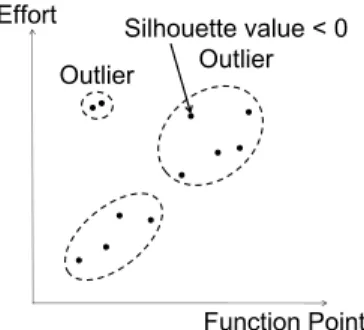
(3) Table 2. An example of outliers in LTS based deletion Effort Residual Effort (estimated) (ordered) …. …. …. … Casem. ym. yˆ m. ( ym  yˆ m ) 2. …. …. …. …. …. n. …. …. …. …. 1. …. adjyi  yi . yˆ a . fp a fp i.  adjy. hSimprojects. 0.25n cases are removed.. (3). h. (4). k. 3. OUTLIER DELETION METHOD An outlier deletion method examines whether a case (project) in a dataset is an outlier or not, and eliminates it from the dataset when it is identified as an outlier. When software development effort is estimated, Cook’s distance based deletion is widely applied before building a linear regression model to eliminate outliers (e.g., [18]). Although Cook’s distance based deletion is used when a linear regression model is built, we also applied it to analogy-based estimation, because it is widely used in many effort estimation studies. Recently, a few outlier deletion methods suitable for analogybased estimation have been proposed. These methods are Mantel’s correlation based deletion [9] and EID based deletion [15]. We applied these methods to analogy-based estimation, to confirm their effects. Past studies have not compared their effects. In addition, we applied our method, neighborhood’s effort based deletion to compare with these methods. We also applied LTS (least trimmed squares) based deletion and k-means based deletion to analogy-based estimation. Although Seo et al. [25] confirmed they were effective toward effort estimation by neural network, it is not clear whether these methods are effective or not toward analogy-based estimation. The outlier deletion methods used in our research are explained below.. 3.1 Cook’s Distance Based Deletion Cook’s distance based deletion is used with multiple linear regression analysis, and identifies an outlier when the case greatly varies the coefficient of the regression model. Cook’s distance indicates how much the residual of all cases varies when a certain case is omitted from model building. A large Cook’s distance means the case greatly affects the model. A case is eliminated from the dataset when Cook’s distance is larger than 4 / n (n is the number of cases in the dataset).. 3.2 LTS Based Deletion LTS (Least trimmed squares) based deletion performs multiple regression analysis, and a case which has a large residual is regarded as an outlier [25]. LTS method is one of the robust regression models. While the ordinary regression model builds a model to minimize the residual sum of the squares, LTS uses up to h-th. Effort. Silhouette value < 0 Outlier Outlier. Function Point. Figure 1. An example of outliers in k-means based deletion residuals (n / 2 < h < n, n is the number of cases) in ascending order, and minimizes the residual sum of squares to build a model. LTS Based Deletion sets h as 0.75n, and 0.25n cases are removed from the dataset, as shown in Table 2.. 3.3 k-means Based Deletion k-means based deletion identifies an outlier based on a clustering result from the k-means method [25]. The k-means method divides data into k clusters, and similar cases are assigned to the same cluster. Data is normalized by equation (1) before clustering, and the value k is set before clustering. k-means based deletion adopts k which minimizes the average silhouette value. The silhouette value is an index which shows whether cases are properly clustered or not, and it is calculated from the distance of each case from the cluster in which the case is included, and the distance from other clusters. The value range of the silhouette value is [-1, 1], and a larger value means that the case is properly clustered. As illustrated in Figure 1, k-means based deletion removes a case when its silhouette value is less than 0, or its cluster has two or less cases.. 3.4 Mantel’s Correlation Based Deletion Mantel’s correlation based deletion identifies an outlier when a set of values of independent variables is similar, but the value of the dependent variable is not similar to other cases. The method was originally proposed in the Analogy-X method [9] designed for analogy-based estimation. The Analogy-X method is (1) delivering a statistical basis, (2) detecting a statistically significant relationship and rejecting non-significant relationships, (3) providing a simple mechanism for variable selection, (4) identifying an abnormal data point (project) within a dataset, and (5) supporting sensitivity analysis that can detect spurious correlations in a dataset. We applied function (4) and (5) as an outlier deletion method. While an ordinary correlation coefficient such as Pearson’s correlation denotes the strength of relationship between two variables, Mantel’s correlation does this between two set of variables (i.e. a set of independent variables and a dependent variable). Mantel’s correlation clarifies whether development effort (the dependent variable) is similar or not, when project attributes such as development size or team size (a set of independent variables) are similar. To determine Mantel’s correlation, each case of Euclidean distance based on the independent variables and the Euclidean distance based on the dependent variable is calculated, and distance matrixes of the distances are made, as shown in Figure 2. Then the correlation coefficient of two matrixes is calculated..

(4) Team Size. C. Table 3. An example of mutually similar cases. D. B A. B. CD. Effort. …. 1. yt … ym …. … … … …. … … … …. Neighborhoods … d …. A. Effort. Caset … Casem …. Function Point B 0.23. B 0.21. C 0.51. 0.36. D 0.63. 0.44. 0.12. C 0.54. 0.32. D 0.66. 0.43. A B C Distance matrix. Based on the Jackknife method, Mantel’s correlation based deletion identifies an outlier when the case greatly affects Mantel’s correlation. That means the case seriously ≤ distorts the relationship between the dependent variable and independent variables. Mantel’s correlation based deletion identifies outliers by the following procedure. 1.. For all projects, Mantel’s correlation ri is calculated by excluding i-th project.. 2.. Average of ri ( r ), and standard deviation of ri (rs) are calculated ( r is the jackknife estimator of Mantel’s correlation). Leverage metric lmi, impact of i-th project on r is calculated by the following equation:. lmi  ri  r 4.. … … … …. 0.13. A B C Distance matrix. 4.. Figure 2. An example of distance matrix used for Mantel’s correlation computation. 3.. … Casem … … Caset … … …. (5). lmi is divided by rs, and when the value (standard score) is larger than 4, the project is eliminated from dataset.. Before calculating Mantel’s correlation, data is normalized using equation (1). Dummy variables made from a categorical variable negatively affect Mantel’s correlation [9]. So we adopted withingroup matrix correlation as proposed in [9].. 3.5 EID based deletion Using EID (Effort Inconsistency Degree), EID based deletion identifies an outlier when the case’s effort is inconsistent with similar cases’ one [15]. The method is designed to apply to analogy-based estimation. EID based deletion identifies outliers by the following procedure. 1.. Neighborhoods of each case are identified by analogy-based estimation, using 10 fold cross-validation.. 2.. Compute the relative error of effort between each case and its nearest case. The 25th percentile of the relative errors is set as the threshold ti.. 3.. For each case in the neighborhoods, check whether Casem included neighborhoods of Caset has neighborhood Caset or not. That is, check whether Casem and Caset are similar to each other. Table 3 shows an example of mutually similar cases.. When Casem and Caset is similar to each other, and Casem is d-th case similar to Caset in the neighborhoods, EID of Casem is calculated by the following equation:.  1 yt  y m   ti   , yt  d  (6) EIDm  EIDm    y  y 1 m  , t  ti   d  yt   In the equation, EIDm is EID of Casem, ti is threshold, yt is effort of Caset, and ym is effort of Casem. 5.. Repeat step 1 to 4 20 times, and cases are removed when their EID is greater than the 90th percentile of the whole EID.. 3.6 Neighborhood’s effort based deletion Our method, neighborhood’s effort based deletion, identifies an outlier when the effort of a project is much higher or lower than other neighborhood projects. As stated in section 2, the procedure of analogy-based estimation consists of range normalization (step 1), neighborhood projects selection (step 2), and estimated effort computation (step 3). When the effort of neighborhood projects is not homogeneous in step 2, estimation accuracy becomes low [23]. Focusing on this issue, our method identifies an outlier in step 2. Analogy-based estimation assumes when the characteristics (independent variables’ values) of project are similar, the effort (dependent variable’s value) is also similar. Our method treats a project as an outlier when the project does not fit this assumption. To identify an outlier, the effort of each neighborhood project is compared to the median of the neighborhood projects’ efforts. However, when the variance of the neighborhood projects’ efforts is large, each project’s deviation from the median effort is also large. So each neighborhood’s effort is standardized before the comparison. Generally, Z-score computation is applied to standardize values. Although Z-score computation assumes a normal distribution, the distribution of neighborhood projects’ effort may not always be a normal distribution. To solve this problem, our method uses robust Z-score computation [22] which does not assume a normal distribution. Robust Z-score computation uses the median and interquartile range instead of the average and standard deviation. Our method eliminates outliers from k neighborhood projects as follows. A neighborhood project’s effort is denoted by yi. Note that yi signifies size adjusted effort (adjyi) when using the size adjustment method. 1.. Median of yi (M) and interquartile range of yi (IQR) is calculated..

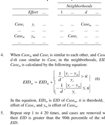
(5) Outlier. y'3. -th. y'2. y'4. 0. th. y'5. Outlier. y'1. Standardized Effort. Figure 3. An example of outliers in neighborhood projects. 2.. Standardized effort y’i is calculated by the following equation (robust Z-score [22]):. yi . yi  M NIQR. (7). In the equation, NIQR (normalized IQR) is equal to 0.7413 IQR. It is equivalent to standard deviation on normal distribution (When the average is 0 and standard deviation is 1, IQR of a normal distribution is 1.34898. Therefore, multiplying IQR by reciprocal of 1.34898 is equivalent to standard deviation). 3.. A project is identified as an outlier and eliminated when the absolute value of y’i is greater than the threshold th (i.e. when the deviation from the median M is greater than th times NIQR). The estimated effort yˆ a is calculated by the following equation:. yˆ a . . hEliminatedprojects. k d. yh. (8). In this equation, Eliminatedprojects denotes a set of k neighborhood projects excluded d outlier projects. We set th as 1.65 (one sided 5% of standard normal distribution). Some studies have pointed out that when the productivity (development size / effort) of neighborhood projects is not homogeneous, the estimation accuracy with size adjustment method becomes low [10][19]. Our method with size adjustment aims to eliminate outliers based on productivity. When size adjustment is used, our method eliminates a project whose adjusted effort adjyi is much higher or lower. From equation (3), adjyi is calculated by multiplying the estimated project’s size fpa by the reciprocal productivity yi / fpi (yi is the effort of a neighborhood project, and fpi is its development size). fpa is same for all neighborhood projects, and therefore it is regarded as a constant. Therefore, adjyi is regarded as productivity in our method. To identify an outlier, Mantel’s correlation based deletion, EID based deletion, and our method focus on cases whose independent variables are similar to each other, but dependent variable is different from each other. A major difference between our method and other methods is that our method is designed to eliminate outliers after selecting neighborhood projects, while other methods are designed to eliminate outliers from the entire dataset before estimation. We examined the effect of the difference on estimation accuracy. An advantage of our method is that it is simpler (less calculation) than other outlier deletion methods.. 4. EXPERIMENT To evaluate outlier deletion methods, we compared the estimation accuracy of analogy-based estimation when each outlier deletion method is applied. We used the ISBSG [8], Kitchenham [12], and. Desharnais datasets [7]. We assumed the estimation point is at the end of the project planning phase. So, only variables whose values were fixed at the point were used as independent variables. We did not compare the deletion methods with case selection methods based on brute-force search or heuristic algorithms [11], because they are rather time-consuming, and therefore their availability is limited.. 4.1 Datasets ISBSG dataset is provided by the International Software Benchmark Standard Group (ISBSG), and it includes project data collected from software development companies in 20 countries [8]. The dataset (Release 9) includes 3026 projects which were carried out between 1989 and 2004, and 99 variables are recorded. The ISBSG dataset includes low quality project data (Data quality ratings are also included in the dataset). So we extracted projects based on the previous study [17] (Data quality rating is A or B, function point was recorded by the IFUPG method, and so on). Also, we excluded projects which included missing values (listwise deletion), because analogy-based estimation and some outlier deletion methods cannot treat a dataset including missing values. As a result, we used 593 projects. The independent variables used in our experiment are the same as the previous study [17] (unadjusted function point, development type, programming language, and development platform). Development type, programming language, and development platform were transformed into dummy variables (e.g. if the variable has n categories, it is transformed into n – 1 dummy variables), because they are nominal scale variables. There is a bit of a debate over the acceptable use of crosscompany datasets such as ISBSG dataset, because due to the disparate collection methods of different organizations, it is possible that cross-company datasets may have some inconsistencies. To lessen the risk, projects which had been collected by almost same collection methods were extracted based on the previous study [17]. Barbara et al. [13] pointed out using cross-company dataset is effective for some companies. The Kitchenham dataset includes 145 projects of a software development company, shown by Kitchenham et al. in their paper [12]. We selected 135 projects which do not include missing values. Three variables (duration, adjusted function point, development type) were chosen as the independent variables, and inadequate variables for effort estimation (e.g. estimated effort by a project manager) were eliminated. Development type was transformed into dummy variables. The Desharnais dataset includes 88 projects in 1980’s, collected from a Canadian company by Desharnais [7]. The dataset is available at the PROMISE Repository [3]. We used 77 projects which do not have missing values. Eight variables (duration, number of transactions, number of entities, adjustment factor, unadjusted function point, programming language, years of experience of team, years of experience of manager) were used as independent variables, and development year and adjusted function point were not used. Programming language was transformed into dummy variables.. 4.2 Evaluation criteria To evaluate the accuracy of effort estimation, we used MRE (Magnitude of Relative Error) [6], MER (Magnitude of Error.

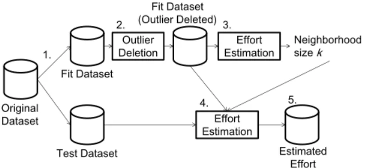
(6) Fit Dataset (Outlier Deleted). 2. Outlier Deletion. 1.. 2.. 3.. Original Dataset. Effort Estimation. Figure 4. Experimental procedure for existing deletion methods. MER . x  xˆ. (9). x x  xˆ xˆ. (10).  x  xˆ  , x  xˆ  0 (11)    BRE   x  ˆ x  x  , x  xˆ  0     xˆ  A lower value of each criterion indicates higher estimation accuracy. Intuitively, MRE means error relative to actual effort, and MER means error relative to estimated effort. However, MRE and MER have biases for evaluating under and over estimation [4][16]. The maximum MRE is 1 even if an extreme underestimate occurs (For instance, when the actual effort is 1000 person-hour, and the estimated effort is 0 person-hour, MRE is 1). Similarly, maximum MER is smaller than 1 when an overestimate occurs. So we adopted BRE whose evaluation is not biased as is both MRE and MER [21], and we evaluated outlier deletion methods based mainly on BRE (MRE and MER were adopted for reference). We did not use Pred(25) [6] which is sometimes used as an evaluation criterion, because Pred(25) is based on MRE and it has also a bias for evaluating under estimation.. 4.3 Experimental Procedure Figure 4 shows the experimental procedure for the existing deletion methods. In the experiment, the fit dataset is used to compute the estimated effort (regarded as past projects), and the test dataset is used as the estimation target (regarded as ongoing projects). Details are as follows: 1.. A dataset is randomly divided into two equal sets. One is treated as a fit dataset, and the other is treated as a test dataset.. 2.. An outlier deletion method is applied to the fit dataset, to eliminate outliers from the fit dataset.. Estimated Effort. Figure 5. Experimental procedure for our method 3.. To decide the neighborhood size k, estimation for the fit dataset is performed, changing k from 1 to 20 (The k was set to a maximum value of 20, since the k over 20 seldom showed high accuracy in a preliminary analysis). After estimation, the residual sum of squares (It is widely used for estimation model selection [16]) is calculated, and the k which shows the smallest residual sum of squares is adopted.. 4.. Estimation for the test dataset is performed. The k adopted in step 3 is used.. 5.. Evaluation criteria are calculated for the actual effort and estimated effort of the test dataset.. 6.. Steps 1 to 5 are repeated 10 times (As a result, 10 sets of fit dataset, test dataset, and evaluation criteria are made).. Relative to the estimate) [12], and BRE (Balanced Relative Error) [20]. Especially, MRE is widely used to evaluate effort estimation accuracy [29] (The residual sum of squares is not widely used for the evaluation). When x denotes actual effort, and xˆ denotes estimated effort, each criterion is calculated by the following equations:. 4.. Effort Estimation With Outlier Deletion Test Dataset. Estimated Effort. MRE . 3.. Original Dataset. 5.. Test Dataset. Neighborhood size k. Fit Dataset. Fit Dataset. 4.. Effort Estimation With Outlier Deletion. 1.. Neighborhood size k. Effort Estimation. Figure 5 shows the experimental procedure for our method. Details are as follows: 1.. A dataset is randomly divided into two equal sets. One is treated as the fit dataset, and the other is treated as the test dataset.. 2.. Estimation for the fit dataset is performed, changing k from 1 to 20. After estimation, the residual sum of squares is calculated, and the k which shows the smallest residual sum of squares is adopted.. 3.. Estimation for the test dataset is performed with our method. The k adopted in step 2 is used.. 4.. Evaluation criteria are calculated for the actual effort and estimated effort of the test dataset.. 5.. Steps 1 to 4 are repeated 10 times.. 5. RESULTS AND DISCUSSION The experimental results are shown in Table 4, Table 5, and Table 6. Each table shows the results for a different dataset. The values of the evaluation criteria are averaged for the 10 test datasets. The top row shows the evaluation criteria when an outlier deletion method is not applied. Other rows show the differences in the evaluation criteria when each outlier deletion method is applied. Negative values mean the evaluation criteria got worse when applying an outlier deletion method. When over 10% improvement of average BRE was observed, BRE was significantly improved (P-value was smaller than 0.05) at least on 5 of 10 test datasets (Wilcoxon signed-rank test was applied for each test dataset). We focused the differences of the evaluation criteria because our major concern is comparative performance of each deletion method..

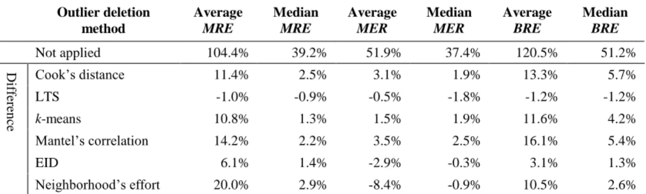
(7) Table 4. Difference of evaluation criteria of each outlier deletion method (ISBSG Dataset) Outlier deletion method Not applied. Average MRE. Median MRE. Average MER. Median MER. Average BRE. Median BRE. Difference. 166.9%. 59.6%. 91.3%. 58.0%. 210.4%. 91.7%. Cook’s distance. 12.2%. -2.9%. -19.1%. -0.8%. -6.0%. -7.4%. LTS. 34.2%. 0.1%. -23.3%. -4.0%. 11.3%. -6.6%. k-means. 0.7%. -3.2%. -20.0%. -2.2%. -17.9%. -10.1%. Mantel’s correlation. 6.1%. -0.7%. -4.0%. 1.3%. 1.8%. 1.2%. EID. 31.0%. 0.9%. -20.9%. -1.2%. 10.0%. -1.7%. Neighborhood’s effort. 47.8%. 5.6%. -16.9%. 0.3%. 28.8%. 4.9%. Table 5. Difference of evaluation criteria of each outlier deletion method (Kitchenham Dataset) Outlier deletion method Not applied. Average MRE. Median MRE. Average MER. Median MER. Average BRE. Median BRE. Difference. 104.4%. 39.2%. 51.9%. 37.4%. 120.5%. 51.2%. Cook’s distance. 11.4%. 2.5%. 3.1%. 1.9%. 13.3%. 5.7%. LTS. -1.0%. -0.9%. -0.5%. -1.8%. -1.2%. -1.2%. k-means. 10.8%. 1.3%. 1.5%. 1.9%. 11.6%. 4.2%. Mantel’s correlation. 14.2%. 2.2%. 3.5%. 2.5%. 16.1%. 5.4%. 6.1%. 1.4%. -2.9%. -0.3%. 3.1%. 1.3%. 20.0%. 2.9%. -8.4%. -0.9%. 10.5%. 2.6%. EID Neighborhood’s effort. Table 6. Difference of evaluation criteria of each outlier deletion method (Desharnais Dataset) Outlier deletion method. Average MRE. Median MRE. Difference. Not applied. 49.5%. 31.1%. Cook’s distance. -0.1% 1.6%. k-means Mantel’s correlation. Average MER. Median MER. Average BRE. 38.3%. 30.2%. -2.9%. -4.1%. -1.4%. -3.3%. -4.9%. -3.8%. -15.8%. -7.4%. -10.9%. -10.3%. -1.2%. -0.5%. -0.5%. -0.5%. -1.4%. -0.5%. -3.2%. -0.9%. -1.8%. -0.9%. -3.9%. -2.2%. EID. 0.8%. -1.2%. -2.0%. -1.8%. -0.8%. -2.6%. Neighborhood’s effort. 0.9%. 0.0%. -2.0%. -0.5%. -1.1%. -1.2%. LTS. 58.3%. Median BRE 36.0%. . Cook’s distance based deletion was effective on the Kitchenham dataset, but it negatively affected estimation accuracy on the ISBSG dataset. On the Kitchenham dataset, it achieved over 10% improvement on the average BRE and over 5% improvement on the median BRE. However, on the ISBSG dataset, the average BRE got over 5.0% worse. On the Desharnais dataset, the average BRE got 3.3% worse.. . k-means based deletion was effective on the Kitchenham dataset, but it negatively affected estimation accuracy on the ISBSG dataset. On the Kitchenham dataset, it achieved over 10% improvement on the average BRE and 4.2% improvement on the median BRE, but on the ISBSG dataset, the average BRE got over 15% worse. On the Desharnais dataset, the average BRE got slightly (1.4%) worse.. . LTS based deletion negatively affected the Desharnais dataset. On the Desharnais dataset, the average BRE got over 10% worse. On the ISBSG dataset, the average BRE got over 10% better, but the median BRE got over 5.0% worse. On the Kitchenham dataset, the average BRE got slightly (1.2%) worse.. . Mantel’s correlation based deletion was effective for the Kitchenham dataset. On the Kitchenham dataset, it achieved over 15% improvement on the average BRE and over 5% improvement on the median BRE. On the ISBSG dataset, the average BRE got 1.8% better, and the median BRE got 1.2% better. On the Desharnais dataset, the average BRE got 3.9% worse, and the median BRE got 2.2% worse..

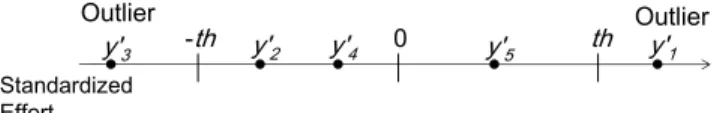
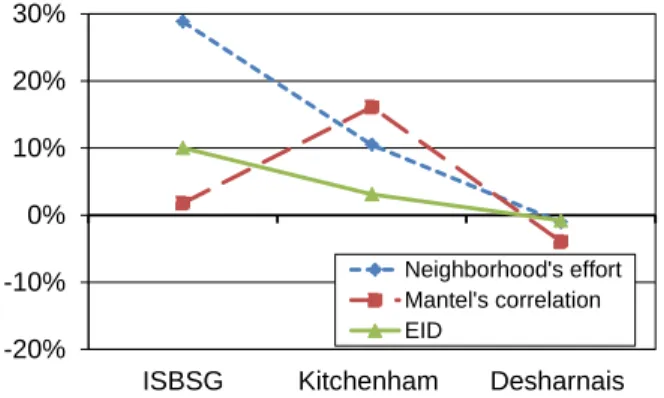
(8) 30%. Cook's distance LTS k-means. 20%. 30%. 20%. 10%. 10%. 0%. 0%. -10%. -10%. Neighborhood's effort Mantel's correlation EID. -20%. -20%. ISBSG. Kitchenham. Desharnais. Figure 6. Average BRE of deletion methods which are not designed to apply to analogy-based estimation. ISBSG. Kitchenham. Desharnais. Figure 7. Average BRE of deletion methods which are designed to apply to analogy-based estimation. . EID based deletion was effective for the ISBSG dataset. On the ISBSG dataset, it achieved 10.0% improvement on the average BRE and the median BRE got slightly (1.7%) worse. On the Kitchenham dataset, the average BRE got 3.1% better, and the median BRE got 1.3% better. On the Desharnais dataset, the average BRE got 0.8% worse, and the median BRE got 2.6% worse.. the average BRE got 6.0% worse. Also, based on MRE, our method seems to have higher performance than Mantel’s correlation based deletion for the Kitchenham dataset. However, MER got worse by our method, and the average and median BRE indicated that Mantel’s correlation based deletion has higher performance than our method for the Kitchenham dataset.. . Our method was effective for the ISBSG dataset and the Kitchenham dataset. On the ISBSG dataset, it achieved over 25% improvement on the average BRE and the median BRE got 4.9% better. On the Kitchenham dataset, the average BRE got over 10% better, and the median BRE got 2.6% better. On the Desharnais dataset, the average BRE got 1.1% worse, and the median BRE got 1.2% worse.. 6. CONCLUSIONS. As shown in Figure 6, deletion methods which are not designed to apply to analogy-based estimation (i.e. Cook’s distance based deletion, LTS based deletion, and k-means based deletion) were effective for one dataset, but they negatively affected estimation accuracy for the other two datasets. Therefore, it is better not to apply these methods to analogy-based estimation, because their performance is not stable. As shown in Figure 7, deletion methods which are designed to apply to analogy-based estimation (i.e. Mantel’s correlation based deletion, EID based deletion, and our method) positively affected two datasets. They negatively affected estimation accuracy for one dataset, but the impact was not very large. So, it is reasonable to apply these methods to analogy-based estimation, because their performance is stable. Especially, only our method showed over 10% improvement of average BRE on two datasets, showing that applying our method to analogy-based estimation is more preferable. Experimental results show it is not appropriate to use only MRE to evaluate outlier deletion methods. Although outlier deletion methods often improved MRE in our experiment, they worsened MER at the same time. This means applying outlier deletion methods caused underestimation on some estimated projects. MRE has biases for evaluating underestimation, and therefore, MRE did not indicate the actual performance of the deletion methods. For example, Cook’s distance based deletion made the average MRE 12.2% better (median MRE 2.9% worse) for the ISBSG dataset. But the average MER was almost 20% worse, and. In this research, we applied outlier deletion methods to analogybased software development effort estimation, and evaluated their effects. In addition, we compared them with our outlier deletion method. While existing deletion methods eliminate outliers from an entire dataset before estimation, our method does this after neighborhood projects are selected by analogy-based estimation. In our method, when the effort of the project is much higher or lower than other neighborhood projects, it is not used for estimation. In the experiment, we estimated development effort using three kinds of datasets collected in software development companies. In the results, Cook’s distance based deletion, LTS based deletion, and k-means based deletion showed unstable performance. Mantel’s correlation based deletion, EID based deletion, and our method showed stable performance. Only our method showed over 10% improvement of the average BRE for two datasets. We conclude that it is reasonable to apply Mantel’s correlation based deletion and EID based deletion to analogy-based estimation, and applying our method is more preferable. As future work, we will apply deletion methods to other datasets and compare their effects to confirm the reliability of our research. Also, we will evaluate effects of deletion methods when missing data techniques are applied.. 7. ACKNOWLEDGMENTS This work is being conducted as a part of the StagE project, The Development of Next-Generation IT Infrastructure, and Grant-inaid for Young Scientists (B), 22700034, 2010, supported by the Ministry of Education, Culture, Sports, Science and Technology. We would like to thank Dr. Naoki Ohsugi for offering the collaborative filtering tool..

(9) 8. REFERENCES [1] Angelis, L., and Stamelos, I. 2000. A Simulation Tool for Efficient Analogy Based Cost Estimation, Empirical Software Engineering 5, 1, 35-68. [2] Boehm, B. 1981. Software Engineering Economics. Prentice Hall. [3] Boetticher, G., Menzies, T., and Ostrand, T. 2007. PROMISE Repository of empirical software engineering data. West Virginia University, Department of Computer Science. [4] Burgess, C., and Lefley, M. 2001. Can genetic programming improve software effort estimation? A comparative evaluation. Journal of Information and Software Technology 43, 14, 863-873. [5] Chan, V., and Wong, W. 2007. Outlier elimination in construction of software metric models. In Proceedings of the 2007 ACM symposium on Applied computing (SAC), Seoul, Korea, March 2007, 1484-1488. [6] Conte, S., Dunsmore, H., and Shen, V. 1986. Software Engineering, Metrics and Models. Benjamin/Cummings. [7] Desharnais, J. 1989. Analyse Statistique de la Productivitie des Projets Informatique a Partie de la Technique des Point des Function. Master Thesis. University of Montreal. [8] International Software Benchmarking Standards Group (ISBSG). 2004. ISBSG Estimating: Benchmarking and research suite. ISBSG. [9] Keung, J., Kitchenham, B., and Jeffery, R. 2008. Analogy-X: Providing Statistical Inference to Analogy-Based Software Cost Estimation. IEEE Trans. on Software Eng. 34, 4, 471484. [10] Kirsopp, C., Mendes, E., Premraj, R., and Shepperd, M. 2003. An Empirical Analysis of Linear Adaptation Techniques for Case-Based Prediction. In Proceedings of International Conference Case-Based Reasoning, Trondheim, Norway, June 2003, 231-245. [11] Kirsopp, C., and Shepperd, M. 2002. Case and Feature Subset Selection in Case-Based Software Project Effort Prediction. In Proceedings of International Conference on Knowledge Based Systems and Applied Artificial Intelligence, Cambridge, UK, December 2002, 61-74. [12] Kitchenham, B., MacDonell, S., Pickard, L., and Shepperd, M. 2001. What Accuracy Statistics Really Measure. In Proceedings of IEE Software. 148, 3, 81-85. [13] Kitchenham, B., Mendes, E., Travassos, G. 2007. Cross versus Within-Company Cost Estimation Studies: A Systematic Review. IEEE Trans. on Software Eng. 33, 5, 316-329. [14] Kitchenham, B., Pfleeger, S., McColl, B., and Eagan, S. 2002. An Empirical Study of Maintenance and Development Estimation Accuracy. Journal of Systems and Software 64, 1, 57-77. [15] Le-Do, T., Yoon, K., Seo, Y., Bae, D. 2010. Filtering of Inconsistent Software Project Data for Analogy-Based Effort Estimation. In Proceedings of Annual Computer Software and Applications Conference (COMPSAC), Seoul, South Korea, July 2010, 503-508.. [16] Lokan, C. 2005. What Should You Optimize When Building an Estimation Model? In Proceedings of International Software Metrics Symposium (METRICS), Como, Italy, Sep. 2005, 34. [17] Lokan, C., and Mendes, E. 2006. Cross-company and singlecompany effort models using the ISBSG Database: a further replicated study. In Proceedings of the International Symposium on Empirical Software Engineering (ISESE), Rio de Janeiro, Brazil, Sep. 2006, 75-84. [18] Mendes, E., Martino, S., Ferrucci, F., and Gravino, C. 2008. Cross-company vs. single-company web effort models using the Tukutuku database: An extended study. The Journal of Systems and Software 81, 5, 673-690. [19] Mendes, E., Mosley, N., and Counsell, S. 2003. A Replicated Assessment of the Use of Adaptation Rules to Improve Web Cost Estimation. In Proceedings of the International Symposium on Empirical Software Engineering (ISESE), Rome, Italy, September 2003, 100-109. [20] Miyazaki, Y., Terakado, M., Ozaki, K., and Nozaki, H. 1994. Robust Regression for Developing Software Estimation Models. Journal of Systems and Software 27, 1, 3-16. [21] Mølokken-Østvold, K., and Jørgensen, M. 2005. A Comparison of Software Project Overruns-Flexible versus Sequential Development Models. IEEE Trans. on Software Eng. 31, 9, 754-766. [22] National Association of Testing Authorities (NATA). 2002. Guide to NATA proficiency testing, Version 2. National Association of Testing Authorities. [23] Ohsugi, N., Monden, A., Kikuchi, N., Barker, M., Tsunoda, M., Kakimoto, T., and Matsumoto, K. 2007. Is This Cost Estimate Reliable? - the Relationship between Homogeneity of Analogues and Estimation Reliability. In Proceedings of the International Symposium on Empirical Software Engineering and Measurement (ESEM), Madrid, Spain, September 2007, 384-392. [24] Selby, R., and Porter, A. 1988. Learning from examples: generation and evaluation of decision trees for software resource analysis. IEEE Trans. on Software Eng. 14, 12, 743757. [25] Seo, Y., Yoon, K., and Bae, D. 2008. An Empirical Analysis of Software Effort Estimation with Outlier Elimination. In Proceedings of the international workshop on Predictor models in software engineering (PROMISE), Leipzig, Germany, May 2008, 25-32. [26] Shepperd, M., and Schofield, C. 1997. Estimating software project effort using analogies. IEEE Trans. on Software Eng. 23, 12, 736-743. [27] Srinivasan, K., and Fisher, D. 1995. Machine Learning Approaches to Estimating Software Development Effort. IEEE Trans. on Software Eng. 21, 2, 126-137. [28] Tosun, A., Turhan, B., and Bener, A. 2009. Feature weighting heuristics for analogy-based effort estimation models. Expert Systems with Applications. 36, 7, 1032510333..

(10) [29] Walkerden, F., and R. Jeffery. 1999. An Empirical Study of Analogy-based Software Effort Estimation. Empirical Soft-. ware Engineering 4, 2, 135-158..

(11)