Evaluation of blind signal separation method using directivity pattern under reverberant conditions

全文

(1)EVALUATION OF BLIND SIGNAL SEPARATION METHOD USING DIRECTIVITY PATTERN U NDER REVERB ERANT CONDITIONS Sαtoshi KURITAt， Hiroshi SARUWATARlt， Shoji KAJITAt， K，αzuyαTAKEDAtαnd FumitαdαITAKURAt ↑Graduate Schoof of Engineering/CIAIR， tCenter for Information Media Studies/CIAIR， Nagoya University Furo-cho， Chikusa-ku， Nagoya， 464-8603， JAPAN E-mail: [email protected]. ABSTRACT. 2. ALGORITHM. This paper describes a new blind signal separation method us ing lhe directivity pattems of lhe microphone a汀ay. In this method， to deal wilh lhe arriving lags among each microphone， the inverses of the mixing matric巴s are calculated in the frequency domain so that the s巴parated signals are mutually independent. Since the cal culations are caπi巴d out in each frequency independently， th巴 fol lowing problems arise: (1) peπnutation of each sound source ， (2) arbitrariness of each source gain. In this paper， we propose a new solution that directivity patterns are explicitly used to estimate the each sound source direction. As the results of signal separation ex periments， it is shown that the proposed method improves the SNR of degraded speech by about 16 dB under non-reverberant condi tion. Also， the proposed method improves the SNR by 8.7 dB when the reverberation time is 184 ms， and by 5.1 dB when the reverberation time is 322 ms.. 2.1. Blind Signal Separation on Microphone Array. In this study， a straight-line aπay is assumed. The coordinates of the elemnents are designated as dk (k = 1，・・. ， K)， and the directions of arrival of mllltiple sound sOllrces are designated asθI (l = 1，"'， L) (see Fig. 1). In general， the observed signals in which multiple source sig nals are mixed linearly are given by the following eqllation in the frequency domain:. where X is the observed signal vector， S is the source signal vec tor， and A is the mixing matrix; these are given as. 1. INTRODUCTION. Blind signal separation (BSS) is the approach to 巴stimate original source signals using only the information of the mixed signals ob served in each input channel. This technique is applicable for the realization of the noise robust spe巴ch recognition and high-quality hands-free telecommunication systems. [n the r巴C巴nt works， as for the BSS based on the independent component analysis [1]， the several methods， in which the inv巴rse of the complex mixing ma trices ar巴 calculated in the frequency domain， have been proposed to deal with the arriving lags among 巴ach element of the micro phone 3πay system [2， 3， 4). Since the calculations 3re carried out in each frequency ind巴pend巴ntly， the following problems arise in these methods: (1) permutation of each sound sourc巴， (2) ar bitrariness of each source gain. To r巴solve these problems， a prト ori assumption of similarity among the envelopes of source signal waveforms must be r巴quired [2， 3) In this paper， we propose a n巴w solution in which the dir巴c tivity pattems of the microphone array system are explicitly used to estimate the each direction of the sound sources [5]. Using this method司 we can resolve both pe打nutation and arbitrariness problems simultaneously without the assumption for the source signal waveforms. In addition， we also show that the proposed method didn't calls巴 heavy degradations of the separation peげor mance compared with thos巴 of the pr巴vious method [2， 3] lInder reverberant conditions The r巴st 01' this paper is organized as follows. In the next sec tion， the formulation for th巴 general BSS problems and the princi ple of the proposed method is explained. In Section 3， the signal separation experiments are performed. Following discussion on the results of the exp巳riments， we give conclllsions in Section 4.. 0-7803-6293-4/00/$10.00@2000. IEEE. ) l (. X=AS，. X. =. S. =. A. =. 1. [X (J)，. . . •. ，. X. K. (fW ，. [SI(J)，，.，SdfW， r A11 (J) • • • A 1L(J) 1 I 1. ・ー A/(L(!) J L AJ..ï (J). (2) (3). (4). We introduce the model to deal with the arriving lags among each 巴lement of the microphone array. In th】IS cas巴， Akμl(f) i恰S，凶i凶s sumed tωo be com甲ple巴Xル-vaωlued. H巴r巴after‘for convenience， we only consider the relative lags among each element with respect to the arrival time 01' the wavefront of the each sound source， and neglec! the pure d巴lay between the microphone and sound source. Also， S is identically regard巴d as the source signals observed at the origin. By ignor川g the effect of the room reverberation， we can rewnte ， the elements in the mixing matrix (Eq. (4)) as the following sim- . ple expression:. Akl(f) = exp(j2πfTkl)，. (Tkl三(l/c) dk sinθ1 ) ，. (5);. 3140 217.

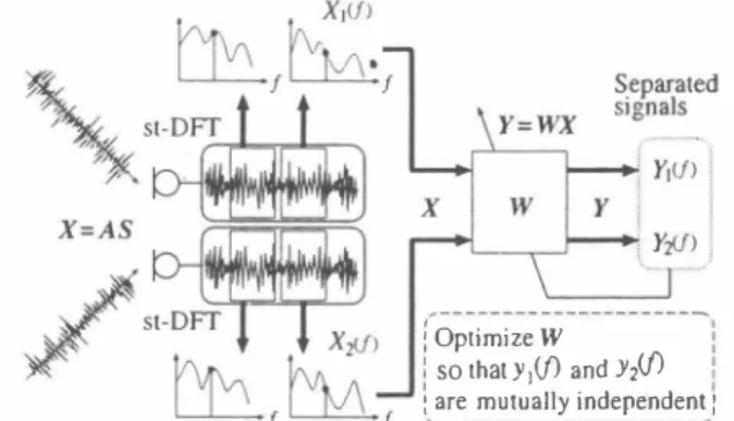
(2) sound. sound source 1. sound source I. 何胃 h日. microphone 1 (d=d J ). microphone k. •••. ! OptimizeW ! so that Y Jの an d YNi. d. (d=dk). Figure 2: Blind signal separation procedure in frequency domain.. Figure 1: Con白guration of a microphone aπay and signals.. SI(1) and S2(1) arises. That is， the separated signal components are possi ble to be permuted every frequency bin， e.g.， in a frequency. Problem 1: The permutation of the source signals. of the mixing matrix， W， so that L time series output Y become mutually independent; this procedure can be given as. y. =. WX. bin of f = h， S1(fl) = SI(h) and S2(h) = S2(h)， and in another frequency bin of f = 12， SI(12) = S2(12). (6). We perform this procedure with respect to all frequency bins. Fi nally， by applying the inverse DFf and the overlap-add technique to the separated time se吋es Y， we reconstruct the resultant source signals in the time domain. As for the calculation of the inverse of the mixing matrix， W， we use the optimization algorithm based on the minimiza tion of the Kullback-Leibler divergence; this algorithm has been introduced by Murata and Ikeda for an on-Iine leaming [2， 3) and modifìed by the authors for an off-line leaming with the stable con vergence [5). The optimal W is obtained by using the following lteratlve equatlOn:. and S2(12)= SI (12). SI(1) and S2(1) are arbitrary. That is， different gains are obtained at the different frequency bins f = h and f = h. Problem 2: The gains of. 2.2.2.. Eq. (9)， SI(1) is given by. Wi+1 = η(diag ((<þ(y)yH))一(φ(y)yH))(wn一 (7) + Wi，. SI(f) = lVll(1)Xl(1) + lVI2(f)X2(1).. l. +3 ， J. 1 ， 1 + exp( _ y(J)). (8). 8). where y(R) and y(J) are the real and the imaginary parts of y， respectively.. 円(f，8) =乞川(f)叫[j27rfdksin8/c]. (11) k=1 This equation shows that the 1 th directivity pattern Ft(f， 8) is pro. 2.2. Signal Reconstruction. In this section， we describe the problems which arise after signal separation shown in Section 2.1， and the solution for these prob lems are newly proposed. Hereafter， we assume the two-channel model without loss of generality， i.e.， K = L = 2. duced to extract the 1 th source signal. Using the directivity pattem Fl(f，θ)， we propose the procedu陀to resolve the Problems 1 and 2 shown in Section 2.2. )， as described below.. 2.2.1. Problems of Source Permutation and Gain Arbitrariness. Step ): We plot the directivity patterns in all frequency bins， e.g.， in the frequency bins of h and 12， directivity patterns are plotted as Fig. 3. We assume that the following separation has been completed in a frequency bin f:. l. A(f)|ーI J.Vll(1) S2(J) I一 I W21(1). Step 2・ln the directivity pattems， directional nul1s exist only in two particular directions. Accordingly， by taking statis tics with respect to directions of the nulls in al1 frequency bins， we can estimate the directions of arrival of the sound sources.. W12(川五(J) 1-1/22(1) I I X2(1). where X1 (1) and X2(1) are the components of the observed sig. nals at the frequency bin f， SI (1) and S2(1) are the components of the estimated source signals， and J.V1k(1) rep問sents the ele ment of the unmixing matrix W. Since the above calculations are carried out in each frequency independently， the following two problems arise (see Fig. 3) .. Step 3: From these directivity pattems， we collect the ones in. which the directional nul1 is steered to the directions of SI and S2 respectively. Here， we decide to collect the direc tivity patterns in which the null is steered to the direction. 3141. 218. (10). This equation shows that the resultant output signals are obtained by multiplying array signals of Xl(f) and X2(1) by the weight 1Ftk(f) and adding them. Thus， from the standpoint of the array signal processing， this operation implies that directivity pattems are produced in the a汀ay system. Accordingly， we calculate direc tivity pattems with respect to lV1k(f) obtained at every frequency bin. The directivity pattern Fl (J， is given by. where ( - ) denotes the averaging operator， i is used to express the value of the i th step in the iterations， and ηis the step size param eter. Also， we defìne the nonlinear functionφ ( . ) as. (R) 1 + exp( - y ). Reconstruction Method Using Directivity Patterns. In order to resolve the problems 1 and 2， we pay attention to the mechanism of the BSS as the aπay signal processing to obtain the separated signals in the acoustical space. For example， from. 1. φ(Y)=. !. : are mutually independent:.

(3) 己目帽。. �I α1FI (/1' 8). 1=/1 F2 (f1' 8). \ν-----ア. source 1 ロ一帽。. 1=ん Pennutation. source 1. source2. a. 〆. source1. source 1. \. sou代e2. 1/ F2(1m，θ2)，. source2. e. source 1. \. よγ. sou代e2. e. rr-=(J 。. εI. Figure 5: Layout of reverberant rooms used in experiments.. ( 12). By substituting W after the above-mentioned modifìcation for Eq. (9). 51 (1) and 52(1)， we can. J. EXPERIMENTS 3.1. Conditions for Experiments. Signal separation experiments were conducted using the sound data convolved with the impulse responses recorded in the six en vironments specifìed by the different reverberation times (RTs). In these experiments， we investigated the performance of separation n d er the di fferent reverberant conditions. A two-element aπay with the interelement spacing of 4 cm is assumed.τ"he speech signals are assumed to arrive from two direc tions， -300 and 400• Two sentences spoken by two male and two female speakers selected from the ASJ continuous speech corpus for research are used as the original speech. Using these sentences， we obtain twelve combinations with respect to speakers and source directions. In these expe吋ments， we used the following signals as the source signals: (1) the original speech not convolved with the impulse responses， (2) the original speech convolved with the im pulse responses recorded in the six environments specifìed by the diff，巴rent reverberation times. Hereafter， we designate the exper iments using th巴 signals described in (1) as the non-reverberant tests， and those of (2) as the reverberant tests. The impulse re sponses are recorded in the roorv shown in Fig. 5. The reverber ation times of the impuls巴responses recorded in the Room 1 and. Loudspea同r1. ildht山2. where θ1 is the estimated direction of the 1 th source. If the source pemlUtation was detected in the previous Step 3， we change αm with βm・. u. ß2FI (f2，8). Room2. tion 01' 52. Without the permutations of the sourc巳s，αm and ßm are described as. and applying inverse 0円to the outputs obtain the source signals correctly. e. 5.87 m. which normalize the gain in the direction of 51， and βI and β2 are the constants which normalize the gain in the direc. ßm =. 1=ん. source2. Figure 4: Resultant directivity pattems after recovery of permuta tions and normalization of gains of separated signals.. Step 4: Problem 2 is. resolved by normalizing the directivity pat tems by the gain in each source direction after the c1assifì cation (see Fig. 4). In Fig. 4，αI and α2 are the constants. 1 / FI (1m，(1)，. source 1. After \ / replaceme�nt V. souにe1. e. of 51 (52) on the right (Ieft) hand side of this fìgure. From this constraint， we replace FI (九θ) with F2(h， B) at the frequency bin of f = h (see Fig. 4). By peげ'orming this procedure， we can resolve the Problem 1.. =. e. ーナゴ. /. Figlire 3: Examples of directivity pattems.. αm. source2. ロaα2F2(/2，8) 。. E1ん，8). ßIF2(/1，8. 1=/1. Room 2 are 184 ms and 322 ms， respectively. Also the impulse responses whose reverberation times are 198 ms司218 ms， 248 ms and 264 ms. are recorded in the Room 1 each other. The remaining conditions 01' the rooms ar巴summarized in Table 1. The analysis conditions in these experiments are shown in Table 2 3.2. Alternative Method for Comparison. In order to compare with the proposed method， we also performed the BSS experiment using the alternative method proposed by Mu rata et al. (2.3) with the modifìcation for an off-line learning Our proposed method is based on the utilization 01' directivity pattems， in contrast， Murata's method is based on the utilization 01' W-1 for the normalization of gains， and a prio吋 assumption 01' similarity among the envelopes of source signal waveforms for the recovery of the source permutation. In this method， the following operatlOns are peけ・'ormed:. (13) = [ZI(f)，...，ZL(J))T=WX，主(1，1) = W-I(Oγ・'，0，ZI(I)，0，・..，O)T， (14) where S( J，1) denotes the component 01' the 1 th 巴stimated source signal in the frequency bin of f. By using both W and W-1， th巴 Z. gain arbitrariness vanishes in the separation procedure. Also. the source permutation can be detect巴d and recovered by measunng the similarity among the 巴nvelopes of S(I，1) between the different frequency bins. 3.3. Results and Discussion. (n order to illustrate the behavior of the proposed aπay for the different RTs， the noise reductioll rate (NRR)， de白n己d as output. 3142. 219.

(4) 18 国てコ. ]. 担14. +. +. AV. AV. 」? AV. 2. .0... .+. 180 200 220 240 260 280 300 320 REVER8ERATION TIME. [ms). Figure 6: Noise reduct】on rates for different reverberant condト tlOns.. �. !ina1-to-noi犯削o (SNR) in dB minus input SNR in dB， is shown .-Fig. 6. These values are taken the average of the whole com・. ∞ ℃. 植岡山ns with respect to speakers and source sentences. SNRs 蜘respond to the objective evaluation score in the case that the t 鈴ppressed signal is regarded as the noise. ln this tìgure， the keys，. 18. 臼Proposed m帥od • Murat自m帥od. 玄14 <0 E H. g 10 に3. 昨30" and“40"， represent the NRRs of the proposed method for �the di附tions of _300 and 400， respectively. Also， the key“ (Sim. ー. 弓6 Q) E. :， ulation)" represents those under non-reverberant conditions.. �. From Fig. 6， in the non刊ve耐rant te山， it can be seen that 16 dB are obtained using the proposed method. mhindu凶that 向 direc附IS of the so肌es are estim批d cor F 柁ctly in the proposed method. However， in the reve巾rant tests，宮 NRRs decrease as the reverberation time increases. Especially， in 批 direction of -30へthe NRR is 8.4 dB in the case that the RT is t 1 84 ms， and the NRR is 4.5 dB in the case that the RT is 322 ms. The main reason for this phenomenon is that since a large number 千of arti白cial sound sources are produced under the reverberant condition， it is hard to suppress the signals which are independent of . the target signal. Figure 7 shows the comparison of the NRRs of the proposed method with those of the conventional Murata 's method under the typical reverberant conditions. These values are taken the aver age of the both direction of sound sources. From this自gure， it is shown that the noise reduction rate is slightly inferior by 0.8 dB to Murata's method in the non-reverberant tests， however， there are no heavy degradations on the proposed method in the rever berant tests， compared with those of Murata's method. The main reason for the degradations in Murata's method is that the output envelopes in the same frequency are similar each other since the inaccurate unmixing matrix is estimated with many components of the cross talk because of the reverberation. Therefore， the re covery of the pe打nutation tends to fail in Murata's method. In contrast， our method didn't fail to recover the source peπnutatJOn because we did not use any informations of signal waveforms but use the directivity pattems only.. 0 z. ì. the NRRs of about. 3. 2 -2. Simulation. RT = 184 ms. RT. =. 322. ms. Figure 7: Comparison of the NRRs of the proposed method with those of Murata's method.. g. i'. beration time is 184 ms. Also， it was shown that NRR decreases as the reverberation time increases， and NRR is 5.1 dB in the case that the reverberation time is 322 ms， however these peげormances are superior to those of the previous Murata's method. 5. ACKNO、-\'LEDGEMENT. This work was suppo口ed by Grant-in-Aid for COE Research (No. lICE2005). 6. REFERENCES. ( 1 ) A. J. Bell and. T. J. Sejnowski， “An infonnation・ maximization approach to blind separation and blind decon volution，" Neural Computation， vol.7， pp. l 129-1159， 1995. (2) N. Murata and S. lkeda，“An on-line algorithm for blind source separation on speech signals，" Proceedings of 1998 ll11ernational Symposium on Nonlinear T heory and its Ap plicatiol1 (NOLTA '98)， voL3， pp.923-926， Sep. 1998. [3] S. Ikeda and N. Murata，“'A method of ICA in time-frequency domain，" Proceedings of lnternational \-\ゐrkshop on Inde pendent Component Analysis and Blind Signal Separation (ICA '99)， pp.365-371， Jan. 1999 [4) P. Smaragdis，“Blind separation of convolved mixtures in the frequency domain，" Neurocomputing， voL22， pp.21-34， 1998. [5) S. Ku吋ta， H. Saruwatari， S. K勾ita， K. Takeda， and F. ltakura， “ Blind signal separatíon using dírectivíty pattern，" Techni.. 4. CONCLUSION. In this paper， a new blind signal separation method using the direc tivity patterns was described. In order to evaluate its effectiveness， the signal separation expe吋ments were performed under reverber ant conditions. As the result， it was shown that the noise reduction rate (NRR) of about 16 dB is obtained under the non-reverberant condition， and NRR of 8.7 dB is obtained in the case that the rever-. cal Report of Japanese Sociery for Artificial Intelligence，. voI.S1G-Challenge-9907， pp.2 1-26， Nov. 1999.. 3143. 220. 6. 。. 1 I I. -30 40. h. .1àble 2: Analysis Conditions in Signal Separation 8 kHz Sampling Frequency Rectangular window Window 32 ms Frame Length I 16 ms Frame Shift 500 Number of 1terations I 4 Step Size Parameter !η= 1.0 X 10-. 10. 40 (Simulation)ー. よ干. 1.4 m 2.2 m 3.3 m. -30 (Simulation)一一. iTAV. 《庄 Z o ト。コ O w Z w ω o z.

(5)