Algorithm of solving second order linear ordinary differential equations and its implementation in REDUCE(Theory and applications in computer algebra)

Algorithm

of

solving

second order

linear ordinary

differential equations

and

its implementation in

REDUCE

L. M. Berkovich

Dept. Algebra and Geometry, Samara State University, Russia

F. L. Berkovich

Dept. Applied Mathematics, Samara State Avia-Space University, Russia

1. Introduction

Theconstruction ofalgorithms for finding formal solutions for some classes of equations

is a main purpose of any constructive theory of ordinary differential equations theory. Explicit formulas are themost important and conclude in itselfall

available

information.

It is necessary to have them also to convince in our physics intuition and to compare different theories including the bounds of their applicability.

Euler, Liouville, Kummer, Jacoby and other mathematicians discovered that the ba-sic method ofintegration and investigation of differential equations is an introducing the convenient changesofvariableswhichreducetheoriginalequations to simplerform. How-ever, they didn’t propose the algorithms for finding this transformations and, as a result, search for suitable substitutions had an euristic character.

Fromthe otherhand, deep relationsbetweenlinear ODE and algebraicequations have

been known for a long time and that lead to the method of factorization of differential

operators. Here many results had a non-constructive character, too.

One of the authors developed in [1] the effective method oftransformation of

differ-ential equations in which there were used both change of variables and factorization of

differential operators.

Thereexist the different approaches forreceivingtheLiouvillian solutions ofODE, i.e.,

those ones that maybe represented in afinite form using elementary, algebraic functions

and quadratures.

An interesting though not complete, review of different methods for receiving the

Liouvillian and otherformal solutions of ODE may be found in [2].

Modemcomputer algebra systems arebecoming thepowerful means ofPC

implemen-tation of the exact methods of ODE investigating and integrating. As a result, many users are able now to use practically those methods available earlier for specialists only.

In this paper we propose our algorithm for finding the general solutions of

nonhomo-geneous second order LODE

$Ly\equiv a_{2}(x)y’’+a_{1}(x)y’+a_{0}(x)y=f(x)$

where coefficients $a_{2},$ $a_{1},$$a_{0}$ belong to some differential field $K$ and they are arbitrary

differentiable functions, possibly, containing parameters. The heart of an algorithm is a

search for variable change that reduces the correspondent homogeneous equation $Ly=0$ to one with constant coefficients.

Algorithm is implemented in computer algebra system REDUCE. 2. Method

2.1. Search for the Kummer-Liouville transformation

Let the equation

$y”+a_{1}(x)y’+a_{0}(x)y=0,$$a_{1}\in C^{1}(I),$$a_{0}\in C(I)$ (1) where $I=\{x|a<x<b\}$ be given. Here for simplicity we assumed $a_{2}=1$

.

Let us apply

here

the Kummer-Liouville $(KL)$

transformation

, i.e. the variable change:

$y=v(x)z(t),$ $dt=u(x)dx$, $u,$$v\in C^{2}(I),$$uv\neq 0,\forall x\in I$

.

(2)

Dueto the St\"ackel-Lietheorem (2) is a most general transformation that keeps the order

and linearity of an equation (1). it is a basic part of the Kummer problem (see [3]) of reduction of(l)to the equation ofaform

$z”(t)+b_{1}(t)z’(t)+b_{0}(t)z(t)=0$, $b_{1}\in C^{1}(J),$$b_{0}\in C(J)$ (3)

where $J=\{t|c<t<d\}$

.

The Kummer problem is always solvable [4] and, therefore, there always exists the

KL-transformation that reduces (1) to (3). However, the problem ofreduction of (1) to

the equation with constant coefficients

$z”(t)+b_{1}z(t)+b_{0}z(t)=0,$ $b_{1},$$b_{0}=const$ (4)

is of the most essential interest.

The KL-transformation may be found using

Lemma 1. The equation (1) may be reduced to (4) by the KL-transformation, for which

the kernel $u(x)$ satisfies to the second order Kumner-Schwarz equation

$\frac{1}{2}\frac{u’’}{u}-\frac{3}{4}(\frac{u’}{u})^{2}-\frac{1}{4}\delta u^{2}=A_{0}(x)$, (5)

where

is a semi-invariant of (1), $\delta=b_{1}^{2}-4k$ is a discriminant of a characteristic equation

$r^{2}+b_{1}r+b_{0}=0$

.

(7)

Then, the multiplier $v(x)$ ofKL-transformation satisfies to the equation resulted

$v(x)=|u|^{-1/2} \exp(-\frac{1}{2}\int a_{1}dx)\exp(\frac{1}{2}b_{1}\int udx)$ (8)

and, moreover, $v(x)$ and $u(x)$ are related by a differential equation

$v”+a_{1}(x)v’+a_{0}(x)v-b_{0}u^{2}v=0$

.

(9)

Lemma 1 allows to find constructive advices on finding $u(x)$

.

Let us consider the equation

$y_{1}’’+a_{1}y_{1}’+a_{01}y_{1}=0,$ $a_{01}=a_{0}(x)-b_{0}u^{2}(x)$ (10)

resulted from (9) after the change $varrow y_{1}$

.

This equation and (1) have the same kernel

$u(x)$ of the KL-transformation.

Since

the coefficient $a_{0}(x)$ due to the formula

$a_{0}(x)=a_{01}(x)+b_{0}u^{2}(x)$ (11)

contains $u^{2}(x)$ as an additive part (up to the multiplicative constant $b_{0}\neq 0$ ), then it is

reasonable to choose candidates for $u(x)$

among

the expressions $a_{0}(x)$ or $A_{0}(x)$ or their

additive parts.

Then the function $w(x)=u^{2}(x)$ must satisfy to the equation

$\frac{1}{4}\frac{w’’}{w}-\frac{5}{16}(\frac{w’}{w})^{2}-\frac{1}{4}\delta w=A_{0}$

.

(12)

Remark: in order to apply this statements, at least one of expressions $\delta$ or $b_{0}$ should

be not zero.

2.2. Factorization

Let us say that the equation (1) admits

_{factorization}

ifits differential operator

$L=D^{2}+a_{1}D+a_{0},$ $D=d/dx$ (13)

may be represented as a product of first order operators

$L=(D-\alpha_{2})(D-\alpha_{1}),$ $\alpha_{1}=\alpha_{1}(x),$$\alpha_{2}=\alpha_{2}(x)$

.

(14)

Here the differential analog of Viet formulas

$a_{1}=-(\alpha_{1}+\alpha_{2}),$ $a_{0}=\alpha_{1}\alpha_{2}-a_{1}’$ (15)

Due to the G.Mammana’s theorem, (1) always admits fact$0$rization.

Lemma 2. The equation (1) may be reduced to (4) by the transformation (2) and admits

factorization

$L=(D- \frac{v’}{v}-\frac{u’}{u}-r_{2}u)(D-\frac{v’}{v}-r_{1}u)y=0$ (16)

where $r_{1},$$r_{2}$ are roots of the characteristic equation (7).

Lemma 9. Zeroes (roots) of factorization may be represented in the form

$\alpha_{1}=-\frac{1}{2}\frac{u’}{u}-\frac{1}{2}a_{1}+\frac{\sqrt{\delta}}{2}u$, $\alpha_{2}=\frac{1}{2}\frac{u’}{u}-\frac{1}{2}a_{1}-\frac{\sqrt{\delta}}{2}u$

.

(17)

This formula connects “zeroes” of factorization with Kummer-Liouville transformation.

Let us now find the feedback of KL-transformation with “zeroes” of factorization.

Using the arbitrariness of determining the characteristic roots $r_{1},$$r_{2}$ , we may require

$r_{1}=r_{2}=0$

.

Then above$fo$rmula takes a form

$\alpha_{1}=\frac{v’}{v}$, $\alpha_{2}=\frac{v’}{v}+\frac{u’}{u}$ (18)

from where

$v=e^{\int a_{1}dx}$, $u=e^{\int(\alpha_{2}-\alpha_{1})dx}$

.

(19)

So, we may formulate

Lemma

_4.

The equatiori (1) by transformation

$y=e^{\int\alpha_{1}dx}$, $dt=e^{\int(\alpha_{2}-\alpha_{1})dx}dx$ ₍₂₀₎

may be reduced to the equation with constant coefficients

$z”(t)=0$

.

(21)

Since in this case the KL-transformation is represented using the “roots” of

factoriza-tion, the elementary procedure for finding factorization may be pointed.

Let us consider the Kummer-Schwarz equation (5) that due to (15) will take a form

$A_{\{}=- \frac{1}{4}(\alpha_{2}-\alpha_{1})^{2}-\frac{1}{2}(\alpha_{2}-\alpha_{1})’$ (22)

from where

$\alpha=\alpha_{2}-\alpha_{1}$

.

2.3. Fundamental system of solutions of LODE

Case 1: equation (1) admits the

_{factorization}

(19).

Lemma 5. Equation (1) has the following fundamentalsystem of solutions (FSS):

$y_{1,2}=u^{-1/2} \exp(-\frac{1}{2}\int a_{1}dx)\exp(\pm\frac{\sqrt{\delta}}{2}\int udx)$, $\delta\neq 0$, (23)

$y_{1}=u^{-1/2} \exp(-\frac{1}{2}\int a_{1}dx),$ $y_{2}=y_{1} \int udx$, $\delta=0$

.

(24)

Case 2: $b_{1}=b_{0}=0$

.

Lemma 6. If the factorization (14)

is

known, then

FSS

as follows:

$y_{1}=e^{\int\alpha_{1}dx}$, _{$y_{2}=y_{1} \int e^{\int(\alpha_{2}-\alpha_{1})dx}dx$}

.

(25)

2.4. Partial solution

Let the nonhomogeneous equation

$y”+a_{1}y’+a+Oy=f(x)$ (26)

be given. If the

FSS

$\{y_{1}, y_{2}\}$ of correspondent equation (1) is known, then the partial

solution $y^{*}$ for Lemma 6 has the form

$y^{*}=-y_{1} \int e^{\int a_{1}dx}y_{2}fdx+y_{2}\int e^{\int a_{1}dx}y_{1}fdx$ (27)

whilefor Lemma 5

$y^{*}= \frac{1}{2\sqrt{-b_{0}}}(y_{1}\int e^{\int a_{1}dx}y_{2}fdx-y_{2}\int e^{\int a_{1}dx}y_{1}fdx)$, $b_{0}\neq 0$

.

(28)

2.5. Semi-invariants and special cases ofa Kummer-Liouville transformation

2.5.1. Semi-invariant $J_{0}$ (invariant by the transformation of dependent

vari-able).

As it was already mentioned above, $J_{0}$ has a form

$J_{0}=a_{0}- \frac{1}{4}a_{1}^{2}-\frac{1}{2}a_{1}’$

.

$IfJ_{0}=const,$ $thentheKL$-transformation will takea form

$y= \exp(-\frac{1}{2}\int a_{1}dx)z,$ _$dt=dx$

.

(29)

Factorization ofoperator $L$ in this case will become commutative:

2.5.2.

Semi-invariant

$J_{1}$ (invariant by the transformation of independent

vari-able).

$J_{1}=a_{0}e^{2\int a_{1}dx}(b_{1} \int e^{-\int a_{1}dx}dx+c)^{2}$

.

(31)

If $J_{1}=const$, then the KL-transformation will take a form

$y=z,$ $dt=- \frac{e^{-\int a_{1}dx}}{b_{1}\int e^{-\int a_{1}dx}dx+c}dx$

.

(32)

We may determine whether $J_{1}$ is a constant or not, using the formula

$\frac{a_{1}}{\sqrt{a_{0}}}+\frac{1}{2}\frac{a_{0}’}{a_{0}\sqrt{a_{0}}}=b_{1}=const$

.

(33)

2.6. Equations solvable algebraically

2.6.1. Exponential solutions

Let the equation $Ly=0$have an exponential solution $y=e^{\lambda x}$, where $\lambda=const$

.

Then the characteristic equation

$r^{2}+a_{1}(x)r+a_{0}(x)=0$ (34)

has

among

its roots $r_{1},$$r_{2}$ not a function but a number

$\lambda$:

$r_{1,2}=- \frac{a_{1}}{2}\pm\sqrt{\frac{a_{1}^{2}}{4}-a_{0}}$

.

(35)

Factorization $L$ takes aform:

$L=(D+a_{1}+\lambda)(D-\lambda)$

.

(36)

2.6.2. Adjoint

equations

By definition, the adjointfor $Ly=0$ equation $L^{*}y=0$ is an equation

$L^{*}y\equiv y’’-a_{1}y’+(a_{0}-a_{1}’)y=0$

.

(37)

It admits factorization

$L^{*}=(D+\alpha_{1})(D+\alpha_{2})$

.

(38)

Let us consider the characteristic equation for adjoint one:

$r^{2}-a_{1}r+a_{0}-a_{1}’=0$

.

(39)

Ifone ofits roots is a number $\lambda$, then the factorization $L^{*}$ takes a form:

$L^{*}=(D-a_{1}+\lambda)(D-\lambda)$

.

(40)

Simultaneously, the factorization $L$ is of the form

2.6.3. Exact equation

If $\lambda=0$, then we have an exact equation, for which the factorization $L$ has a form

$L=D(D+a_{1})$

.

(42)

3. Implementation

The

REDUCE program SOLDE

which implements the algorithm described above,has

the following main characteristics:

INPUT: a2 al $a0,f$ $/{}_{0}Coefficients$ _of given equation

OUTPUT: u.v, $\iota/.variable$ change

bl $bO$, $’/*coefficients$ of reduced equation

alfal alfa2, $|/.coefficients$ of factorization

yl,$y2$, $’/.FSS$

yp $’/.partial$ solution for nonhomogeneous ODE

The method is, really, an algorithm itself, so the computerprogram SOLDEwritten in computer algebra system REDUCE, follows to the second part of this paper in detail, so

there is no need to describe it here. It should be pointed only, that for make the program

more convenient for users and faster the second author decided to include the coefficient

$a_{2}$ under consideration. It may be explained by the fact that sometimes, that was proved

theoretically, the candidate for $u(x)$ may be taken from $u(x)=1/q(x)$, where $q(x)$ is a $a_{2}(x)$ or its multiplicative part.

Program SOLDEwastested on hundredsof equations and it had success in 75% cases.

Failure in the left 25% are caused by two reasons: 1) theother important transformation,

ofEuler-Imshenetsky-Darboux,wasnotincludedto the

program

yet,thoughthere already exist all thenecessaryformulas for its application here, and 2) the algorithm doesn’t work

when $b_{1}=b_{0}=0$

.

For illustrate the current possibilities ofthis

program,

let us name the equations from

the demonstration file:

$***$ I.Equations with constant _coefficients $***$

$Y’ l+A*Y’+B*Y=F(X)$ $Y’ l+A*Y)+A*A/4*Y=F(X)$

$***$ II. Euler’$s$ equations $***$

$Y^{l}$ $+A/X*Y’+B/(X*X)*Y=F(X)/(X*X)$

*** III.Equations _of a _form : $***$

$Y’)+A1(x)*Y^{l}=F(X)$

$***$ _{IY.Equations with exponential coefficients} $***$

$Y’+A*Y)+B*E**(2*A*X)*Y=F(X)$

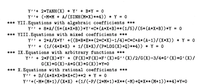
$***Y.Equations$ with trigonometrical functions $***$

$Y’$ $‘+2*A*C0T(A*X)*Y)+(B*B-A*A)*Y=0$

$Y$’ $‘+(M*M+A/SIN(2*M*X)**2)*Y=0$

$Y$‘ $’+2*TANH(X)*Y$’ $+B*Y=0$

Y) $‘+(-M*M+A/(SINH(M*X)**4))*Y=0$

$***YII.Equations$ with algebraic coefficients $***$

$Y^{\prime l}+8*A/(5*(A*X+B))*Y^{l}+C*(A*X+B)**(1/5)/(5*(A*X+B))*Y=0$

$***YIII.Equations$ with mixed coefficients $***$

$Y”+2*A/X*Y’+((B*B*E**(2*C*X)-1/4)*C*C+A*(A-1)/(X*X))*Y=0$ $Y))+(1/(4*X*X)+1/(X*X)/(P*LOG(X)+Q)**4))*Y=0$

$***$ IX.Equations with arbitrary functions $***$

$Y^{l}$ $+2*F(X)*Y^{l}+(F(X)*F(X)+F(X)+G)(X)/2/G(X)-3/4*G^{l}(X)*G(X)/$

$G(X)*G(X)-A*G(X)*G(X))*Y=0$

***X.Equations with rational coefficients $***$

$Y^{ll}+D/(A*X*X+B*X+C)**2*Y=0$

$Y))+(-M*(M+1)/(X*X)+(1/(-P/(2*M+1)*X**(-M)+Q*X**(M+1))**4)*Y=0$

High efficiency of this implementation is caused by the fact that entire package was

developed around the procedure

SOLDE

which allows to the user to investigate his

ODE

from different sides, and even the

program

doesn’t give an answer itself, it often helps

the user in finding the approaches to his equation making more effective and faster his operations and testing his propositions. Thus, each ODE maybe investigated during the

whole session by the procedures shown in Table 1.

Table 1. Procedures in the package.

2: $|/_{0}Specia1$ case of this equation with $a=1$ was solved by Kovacic [5]

$|/.in$ another way

solde$(x^{\sim}2,0,-a*x+3/16 , 0)$ ;

$*Summary$ of the $operations*$

$***************************************************************$ $*The$ equation was: $(X^{2})*y^{l}$ $‘+$ (0)_$*y)+$ $( - ——-)*y\underline{1}\underline{6}*\underline{A}*\underline{X}-\underline{3}=0$

16

$——-\underline{1}\underline{6}*\underline{A}*\underline{X}-\underline{3}_{-}$

$*The$ semi-invariant by dependent variable: $J0=$

$16*X^{2}$

1/4 ₁

$*The$ transformation: $y=$ (X )$*z$, dt $=$ (———) dx

SQRT (X) $*$ leads to $z’$ ) _{$(t)+(0)*z^{J}(t)+$}

$( -A)*z(t)=0$

$*The$ factorization: $4*SQRT(A)*X+$ SQRT(X) $*$

$L=(D-(————————))$

$(D-($ $4*SQRT(X)*X$ $4*SQRT(A)*X+$ SQRT(X)

$———————–))$

$4*SQRT(X)*X$

$*Fundamental$ system of solutions of $Ly=0$:

1/4 $2*SQRT(X)*SQRT(A)$ $Y1=$ X $*E$ 1/4 $x$

$Y2=——————–$

$2*SQRT$(X)*SQRT(A) $E$ $**************************************************************$

The previous version of the

program

is described in [6].

References

[1] BerkovichL.M., Factorizationand

_{Tmnsformations of}

Ordinary

_Differential

Equations,

Sara-tov Univ. Publishers, Saratov, 1989 (in Russian)

[2] Singer M. F., FormalSolutions

_of

_Differential

Equations, J. Symb. Comp., 1990, 10, 59-94

[3] Boruvka 0., Lineare

_{Differential Tmnsformationen}

2. Ordnung, Berlin, 1967

[4] Berkovich L. M.,

_{Transformations}

_of

Linear Ordinary

_Differential

Equations, Kuibyshev

State Univ, 1978 (in Russian)

[5] Kovacic J., AnAlgorithm

_for

Solving Second Order Linear Homogeneous

_Differential

equa-tions, J. Symb. Comp., 1986, 2, 1

[6] Berkovich L. M., Gerdt V. P., Kostova Z. T., Nechaevsky M. L., Second Order Reducible