Lectures on Pleating Coordinates for Once Punctured Tori (Hyperbolic Spaces and Related Topics)

Lectures

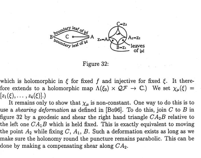
on

Pleating Coordinates for

Once

Punctured

Tori

Caroline Series

Mathematics

Institute, Warwick University

Coventry CV4

$7\mathrm{A}\mathrm{L}$

,

UK

cms@maths.warwick.ac.uk

Preface

Pleating coordinate theory is a novel approach to understandingdeformation spaces ofholomorphic families of Kleinian groups, introduced in recent years

by the author and Linda Keen. The key idea is to study deformation spaces

via the internal geometry of the associated hyperbolic 3-manifold, in

partic-ular, the geometry of the boundary of its

convex

core.

This allows one to

relate combinatorial, analytical and geometrical data in hitherto unobserved

ways. One important outcome is to give algorithms enabling

one

to compute

the exact position of the deformation space,

as a

subset in $\mathbb{C}^{n}$

.

The idea is

loosely similar to finding the Mandelbrot set by drawing its external rays. It

is based

on

the observation that there is a close link between the geometry of boundary of the

convex

core

and the complex analytic trace

or

length function of its bending lamination:

a

geodesic axis is

a

bending line implies

that the corresponding group element has real $\mathrm{t}\mathrm{r}\mathrm{a}\mathrm{c}\mathrm{e}$. In these lectures, we

develop the theory

as

it relates to

once

punctured tori. We show that,from

this simple startingpoint,

one can

give

a

complete description of the position

of the pleating varieties, that is, the loci

on

which the projective class ofthe

bending

measure

of each ofthe two components of the

convex

hull boundary

is fixed. We then discuss how this enables

one

to compute an arbitrarily

of groups, and conclude with a detailed description of how to compute the

exact image of any embedding of the space of

once

punctured torus groups

into $\mathrm{P}\mathrm{S}\mathrm{L}(2, \mathbb{C})$

.

The lectures

on

which these notes

are

based

were

given in Osaka City

University in July

1998.

They

are

an

exposition of material which has been

developed in

a

series of papers by the author and L,Keen. _{We have not}

al-tered the informal style of the lectures: this account is intended

as

a

short

user friendly guide. There are certainly many inaccuracies, some deliberate

in the interests of brevity and

some

inadvertent. Detailed proofs

are

to be

found in the papers of Keen and Series, especially in [KS98] and [KS93].

Useful background may also be found in

an

earlier series oflectures given by the author in Seoul, Korea [Se92]. Since these lectures

were

given

we

have revised the preprint [KS98] to correct a gap in the proofof the limit pleating theorem 3.11, and to give

a

shortened proof of the real length lemma 3.8.

These changes have been incorporated into these notes. Since otherwise the two versions

are

largely the same,

we

refer mainly to the original

ver-sion [KS98]. Where there is substantial difference,

we

refer to the revised

version

as

$[\mathrm{K}\mathrm{S}98\mathrm{a}]$.

The computer graphicshave been done at various times by various people,

notably David Wright, Ian Redfern and Peter Liepa. We thank them for

permission to include them here. The author would especially like to thank

Yohei Komorifor organizing the Osakaconference to give her the opportunity

of presenting this work, and Hideki Miyachi, without whose help the notes

would probably not have

seen

the light of day. Most of all, it is

a

pleasure to thank Komori for his untiring interest in all aspects of this work.

Contents

Lecture 1: Introduction.

..

..

.

.. ...

....

.

.

..

... .

.

.

..

.

..

..

.

.

...

.

..

.

...

.

3

Lecture 2: Convex hull boundary: rational

case.

.

... ...

...

..

.

..

15

Lecture 3: Irrational laminations...

.

.

..

...

...

...

26

Lecture

4: One dimensional examples...

...

..

.

.

...

... ...

..

35

Lecture 5: Main technical theorems... 43

Lecture 1:

Introduction and

discussion

of

several

examples

In this lecture we introduce quasifuchsian space

_for

once punctured tori and

de-scribe the general problem we aim to solve in these notes. We give examples

of

some

_{families of}

Kleinian groups we shall be studying and discuss the

Mumford-Wright exploration

_of

parameter space which provided the original motivation

_for

our approach. We conclude with a

_brief

introduction to the hyperbolic convex hull.

The general setting for these lectures is that of

a

holomorphic family

_of

Kleinian groups. Recall that

a

Kleinian group $G$ is

a

discrete subgroup of

$\mathrm{P}\mathrm{S}\mathrm{L}(2, \mathbb{C})$

.

Its action

on

the Riemann sphere

$\hat{\mathbb{C}}$

decomposes into the regular

set $\Omega$,

on

which the elements of _$G$ act properly discontinuously and form a

normal family, and the limit set $\Lambda=\hat{\mathbb{C}}-\Omega$

on

which the $G$-action is minimal,

that is,

on

which every orbit is dense. By the

_Ahlfors

Finiteness Theorem,

if $G$ is finitely generated then $\Omega/G$ is

a

finite union of Riemann surfaces of

finite genus with finitely many punctures. In these lectures we concentrate

especially

on

quasifuchsian

once

punctu$7^{\cdot}ed$ torus groups. For these groups

$\Omega$ has exactly two connected components, $\Omega^{+}$ and $\Omega^{-}$, each of which is

G-invariant and simply connected, such that $\Omega^{\pm}/G$

are

both punctured tori.

The limit set $\Lambda$ is a topological circle. Such

a

group $G$ is

a

free group

on

two generators $\mathrm{A},$ $B$ whose commutator $[A, B]=ABA^{-1}B^{-1}$ is necessarily

parabolic. The generators

are

represented by generating loops $\alpha,$ $\beta$

on

$\Omega^{\pm}/G$

so that $\langle\alpha, \beta\rangle=\pi_{1}(\Omega^{\pm}/G)$. (Note however that the relative orientation of$\alpha$

and $\beta$ on _{$\Omega^{+}/G$} and _{$\Omega^{-}/G$} is opposite.)

By Bers’ Simultaneous

_Unifo

rmization Theorem, given any two (marked)

complex structures $\omega^{\pm}$

on

a once punctured torus, there exists aquasifuchsian

once

punctured torus group $G$ for which $\Omega^{+}/G=\omega^{+},$ $\Omega^{-}/G=\omega^{-}$ This

group is unique up to conjugation in $\mathrm{P}\mathrm{S}\mathrm{L}(2, \mathbb{C})$.

A holomorphic family of finitely generated Kleinian groups $G=G(\xi)$,

$\xi\in \mathbb{C}^{n}$, is

a

family of Kleinian

groups

$G=\langle g_{1}(\xi), \ldots , g_{k}(\xi)\rangle$ for which the

generators $g_{i}(\xi)$

are

holomorphicfunctions of$\xi$

on some

open set $U\subseteq \mathbb{C}^{n}$

.

By

a

result of Sullivan, if$U\subset \mathbb{C}^{n}$ is open and all the representations $G_{0}arrow G(\xi)$

are

faithful (for

some

fixed

group

$G=\langle g_{1}^{0},$

$\ldots$ ,

$g_{k}^{0}\rangle$), then $G(\xi)$ is

quasi-conformally equivalent to $G_{0}$. In the

case

of quasifuchsian

once

punctured

torus groups, after correct normalization, we find $n=2$

.

This corresponds

to the fact that the Bers parameters $\omega^{\pm}$

are

each points in the upper half

shall always denote by $\mathcal{T}$. We denote a

more

general holomorphic family by $\mathrm{D}\mathrm{e}\mathrm{f}(G)$

.

Exercise Do

a

dimension count on $G=\langle$$A,$ $B|[A,$$B]$ is parabolic $\rangle$ to

“verify” $n=2$ is _correct.

The Problem In these notes, $QF$ always refers to the space of

once

punc-tured $\mathrm{t}\varphi$

rus

groups. Our aim

iri

these lectures is to solve the following

prob-lem:

Given

some

specific set

_of

holomorphic parameters $\xi\in \mathbb{C}^{2}$

for

groups $G=G(\xi)=\langle$$A,$ _$B|[A,$$B]$ is $\mathrm{p}\mathrm{a}\mathrm{r}\mathrm{a}\mathrm{b}\mathrm{o}\mathrm{l}\mathrm{i}\mathrm{c}\rangle$ ,

describe exactly how to compute quasifuchsian space

$QF=$

{

$\xi\in \mathbb{C}^{2}|G(\xi)$ is

a

quasifuchsian

once

punctured torus $\mathrm{g}\mathrm{r}\mathrm{o}\mathrm{u}\mathrm{p}$

}

$\subset \mathbb{C}^{2}$

In $particular_{r}$

find

$\partial QF\subset \mathbb{C}^{2}$

By Bers’ theorem, we know that $Q\mathcal{F}^{\cdot}$ is biholomorphically equivalent to $\mathbb{H}\cross \mathbb{H}$. However this gives

no

information about the shape of $QF$ in $\mathbb{C}^{2}$

.

We have two further useful pieces of information, namely the position of

Fuchsian space $F$ for which $\omega^{+}=\overline{\omega^{-}}$ (the complex conjugate of

$\omega^{-}$), $\Omega^{\pm}$

are round discs and $\Lambda$ is a round circle; and the nature of a dense set of

boundary points of $QF$ called cusps. Before discussing these further, let us

look at

some

specific examples of the kinds of holomorphic parameters we

have in mind.

$\mathrm{J}\emptyset \mathrm{r}\mathrm{g}\mathrm{e}\mathrm{n}\mathrm{s}\mathrm{e}\mathrm{n}$ Parameters for $Q\mathcal{F}$

.

One

can

normalize

so

that

$\mathrm{A}=(^{u-v/w}u$ $v/w^{2}v/w$

)

$B=$

$[A, B]=$

where $u,$ $v,$$w\in \mathbb{C}$ with $u^{2}+v^{2}+w^{2}=uvw$. This relation is called the

Markoff

equation and follows from the trace identities in $\mathrm{P}\mathrm{S}\mathrm{L}(2, \mathbb{C})$

.

In this

case

$G=\langle A, B\rangle$ is Fuchsian (and hence in particular discrete) if and only if

$u,$ $v,$ $w\in \mathbb{R}$. Note $u=\mathrm{T}\mathrm{r}A,$ $v=\mathrm{T}\mathrm{r}B,$ $w=\mathrm{T}\mathrm{r}$AB.

Button Parameters. A variant on the above is the following

$A=(^{(1+z^{2})/w}z$ $wz)$ $B=(^{(1+w^{2})/z}-w$ $-wz)$ $[A, B]=(_{0}^{-1}$ $-u-1)$

Here $u=2(1+z^{2}+w^{2})/zw,$ $z,$$w\in \mathbb{C}$ and

once

again, $G$ is Fuchsian if and

only if $z,$$w\in \mathbb{R}$.

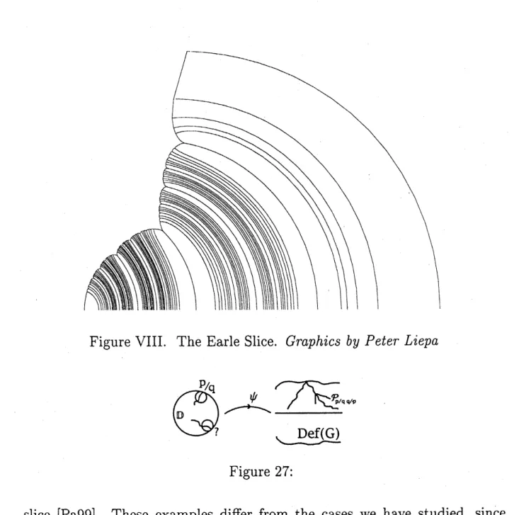
The Earle slice of $QF$

.

$([\mathrm{K}\mathrm{o}\mathrm{S}98\mathrm{a}])$ This is a one-complex dimensional

slice of $Q\mathcal{F}$ in which $\Omega^{+},$ $\Omega^{-}$ are required to be conformally isomorphic under

the rhombic symmetry $$ which sends $\mathrm{A}arrow B,$ $Barrow A$. It extends the

rhom-bus line $|\tau|=1$ in the classical upper half plane picture of the Teichm\"uller

space of a torus holomorphically into $QF\subset \mathbb{C}^{2}$

.

The parameterisation is:

$A=$

(

$\frac{d^{3}}{2d^{2}+1,d}$

)

$B=(_{-}^{\frac{d^{2}+1}{\frac{2d^{2}+1d}{d}}}$ $- \frac{d^{3}}{2d^{2}+1,d})$

Here $d\in \mathbb{C}$. The conformal involution $$ is normalised

so

that

$(z)=-Z$

.

We have $A^{-1}=B$ and

once

again, $G\in F$ if and only if $d\in \mathbb{R}$. We shall

come back to this example in lecture 4.

The Maskit embedding of $\mathcal{T}$

.

This is a 1-dimensionalholomorphic slice

on

$\partial Q\mathcal{F}$ consisting of groups for which the generator $A$ is pinched to a

parabolic (a so called cusp group). This is the slice whose study led to

the first results on pleating coordinates in [KS93]. It

was

first introduced by

David Wright in [Wr88].

$A=$

$B=-$

$\xi\in \mathbb{C}$

Here $\Omega^{+}/G$ is a

once

punctured torus while $\Omega^{-}/G$ is

a

3-times punctured

sphere. Since the Teichm\"uller space of a 3-times punctured sphere is a single

point, we have $\mathrm{D}\mathrm{e}\mathrm{f}(G)=\mathcal{T}=\mathbb{H}$. The parameters were chosen

so

that the

map $(\mathbb{H}, \tau)arrow(\mathrm{D}\mathrm{e}\mathrm{f}(G), \xi)$ should take the simplest possible form. This is

1.1

Exploration

of

$Q\mathcal{F}$

and the

Mumford-Wright

Pro-gramme.

In the early $1980’ \mathrm{s}$, David Mumford, David Wright and Curt $\mathrm{M}\mathrm{c}\mathrm{M}\mathrm{u}\mathrm{l}\mathrm{l}\mathrm{e}\mathrm{n}$

em-barked on computer explorations of $QF$

.

In particular, they plotted many

limit sets and looked for cusp groups on $\partial Q\mathcal{F}$. A cusp is a group in which

an element representing a simple (non-self intersecting) curve

on

the torus

becomes parabolic. One can think as moving towards a cusp on $\partial QF$ as

the process of shrinking a simple closed loop on one or other of the surfaces

$\Omega^{\pm}/G$. (This

usage

is not to be confused with a cusp in the sense of a

punc-ture on a hyperbolic surface; in the one case it is a missing point and in the

other, by extension, it refers to the whole group.) Later, $\mathrm{M}\mathrm{c}\mathrm{M}\mathrm{u}\mathrm{l}\mathrm{l}\mathrm{e}\mathrm{n}$ proved

that cusps are dense on the boundary of every Bers slice in $QF,$ $[\mathrm{M}\mathrm{c}\mathrm{M}91]$

.

David Wright made a more systematic study of the Maskit embedding $\mathcal{M}$

described above. His plan was:

$\bullet$ Enumerate homotopy classes ofsimple closed curves on the once

punc-tured torus.

$\bullet$ Find representativesofthese

curves

as elements in $G$ and computetheir

traces as functions of $\xi$

.

$\bullet$ Find points where the traces $\mathrm{a}\mathrm{r}\mathrm{e}\pm 2$ (parabolics).

Note the problem with the last point: there may be many places where

an element is parabolic, but we cannot conclude that the group is necessarily

on $\partial Q\mathcal{F}$or $\partial \mathcal{M}$. In general, such a group may not even be discrete.

Since Wright’s enumeration of curves underpins much of what we are

about to do, we explain it briefly here. Let $S$ denote a (topological)

unpunc-tured torus and $\Sigma$ a torus with a puncture. Both have marked generators

$A,$ $B$

.

The fundamental group $\pi_{1}(S)$ is the free abelian group $\mathbb{Z}^{2}$ while

$\pi_{1}(\Sigma)$

is $F_{2}$, the free group on two generators. For each $p/q\in\hat{\mathbb{Q}}=\mathbb{Q}\cup\{\infty\}$ (we

allow $q=0\Leftrightarrow\infty\in\hat{\mathbb{Q}}$), the homotopy class $A^{-p}B^{q}$ represents a simple

closed loop on $S$. This loop is also simple on $\Sigma$ and hence corresponds to

some element (conjugacy class) $W_{p/q}$ in $\pi_{1}(\Sigma)$

.

By considering the action of

the mapping class group on $S$ and $\Sigma$, one can show that all simplehomotopy

classes on $\Sigma$ arise in this way. The arrangement of these loops is shown in

Figure 1:

$A^{-p}B^{q}$ on $S$, which we can think of as a line of rational slope in the plane

projected onto $S$.

Exercise Find the slope on $\mathbb{R}^{2}$ of line which projects to $A^{-P}B^{q}$

.

Remark It is well known that on a hyperbolic surface, each free homotopy

class contains a unique geodesic. Therefore, given a hyperbolic metric on $\Sigma$,

these classes represent exactly the simple closed geodesics of $\Sigma$

.

Notice that successive $p,$ $q$ curves can be enumerated by Farey addition

$\frac{p}{q}\oplus_{F}\frac{r}{s}=\frac{p+r}{q+s}$, whenever ps–rq $=\pm 1$.

Wright showed that cyclically reduced words in $F_{2}$ corresponding to $A^{-p}B^{q}$

could be found inductively by the following process, see also [KS93]$)$.

$W_{0/1}=B,$ $W_{1/1}=A^{-1}B,$ $\mathrm{T}/V_{1/0}=|/V_{\infty}=A^{-1}$

$W_{(p+r)/(q+s)}=W_{r/s}\nu V_{p/q}$ if ps-rq $=-1$.

Note the unexpected order in the

d.efinition

of $\nu V_{(p+r)/(q+s)}$.

Using the trace identity Tr$XY=\mathrm{T}\mathrm{r}X$ Tr$Y-\mathrm{T}\mathrm{r}XY^{-1}$ (which holds for

$\bullet$ Tr $\nu V_{p/q}$ is a polynomial of degree $q$ in $\xi$

.

$\bullet$ Tr $W_{p/q}=(-i)^{q}(\xi-2p/q)^{q}+O(\xi^{q-2})$, where $O(\xi^{q-2})$ denotes terms of

order $\leq q-2$

.

Exercise Do this. (See [KS93,

_{\S 3.2].)}

Thus in general, the equation for the cusp group in which $\nu V_{p/q}$ is pinched

is Tr$W_{p/q}(\xi)=\pm 2$

.

This has $2q$ roots, of which, however, only one is a

discrete

group

on $\partial M$ [KMS93]. (Actually two, since to get a unique copy of $\partial \mathcal{M}$ we should normalize with

${\rm Im}\xi>0$, see 1.3 below.) In the special case

$q=1$, however, there is a unique root with ${\rm Im}\xi>0$; these are the points

$\xi=2n+2i,$ $n\in \mathbb{Z}$ and correspond to cusps in which both $A$ and $A^{-n}B$ are

parabolic (so $\Omega^{+}/G$ and $\Omega^{-}/G$ are both 3-times punctured spheres). At the

point $\xi=2n+2i$, notice that Tr$W_{n/1}(\xi)=2$

.

Wright plotted these points and then proceeded to find roots of Tr$\nu V_{p/q}(\xi)=$

$2$ by Newton’s method and interpolation, using therecursion describedabove.

The result is shown in Figure I: it looks very like a boundary $\partial \mathcal{M}$!

He also made pictures of the limit sets of these special groups, see Figure

II. Notice the two families of black and white circles, which correspond to

the two thrice punctured sphere subgroups in $\Omega^{+}/G$ and $\Omega^{-}/G$

.

These

pic-tures were the starting point of [KS93]. After much computation and

explo-ration, Keen and the author proposed plotting the branches of Tr $\nu V_{p/q}>2$,

Tr $W_{p/q}\in \mathbb{R}$ moving away from the cusp. The result is shown in Figure III.

Corresponding limit sets are shown in Figures IV and V in which you can see

that the

_tange,nt

$\mathrm{c}\mathrm{i}‘ \mathrm{r}\mathrm{c}\mathrm{l}\mathrm{e}\mathrm{s}$ in Figure II have opened so they now overlap.

No-tice that the real trace lines of Figure III have remarkable properties, which would certainly not be expected of the real loci of an arbitrary family of

polynomials (or even this family ifthe lines through other solutions to Trace

$=\pm 2$ were chosen.) In particular:

1. they are $\mathrm{p}\mathrm{a}\mathrm{i}\mathrm{r}\mathrm{w}\mathrm{i}\mathrm{s}\mathrm{e}\backslash$ disjoint;

2. they end in “cusps”;

3. they contain no critical points;

4. they are asymptotic to a fixed direction at $\infty$;

At this stage

none

ofthese properties could be either explained or proven.

The key turned out to be to study the action of $G$

on

hyperbolic 3-space $\mathbb{H}^{3}$,

in particular, on the boundary of the

convex

hull. This also eventually led

to our method of drawing the parameter space $Q\mathcal{F}$.

For the rest of this lecture

we

shall discuss this

convex

hull.

1.2

The

Boundary

of the Hyperbolic

Convex

$\mathrm{H}\mathrm{u}\mathrm{l}\mathrm{l}$

Recall that a Kleinian group $G$ acts not only on the Riemann sphere $\hat{\mathbb{C}}$ but

also

on

on hyperbolic 3-space $\mathbb{H}^{3}$, which

can

be regarded

as

the interior $\mathrm{B}^{3}$

of the Riemann sphere $\hat{\mathbb{C}}$

. The quotient $\mathbb{H}^{3}/G$ is a hyperbolic 3-manifold; in

the case of a quasifuchsian

once

punctured torus group, it is homeomorphic

to $\Sigma\cross(0,1)$. The surfaces $\Omega^{\pm}/G$ compactify the 2-ends of $\mathbb{H}^{3}/G$

so

that

$(\Omega\cup \mathbb{H}^{3})/G\simeq\Sigma\cross[0,1]$.

The convex hull

or convex

core $C$ (Nielsen region) of$\mathbb{H}^{3}/G$ is the smallest

hyperbolic closed set containing all closed geodesics of $\mathbb{H}^{3}/G$. If $G$ is

Fuch-sian, $\mathrm{a}_{\iota}^{1}1$ of these

are

contained in a single flat plane, otherwise we get the

picture shown in figure 2.

$\mathrm{G}$ quasituchsian

(Note $\Omega^{+}/\mathrm{G}\neq\Omega^{-}/\mathrm{G}$

as

conformal tori)

Figure 2:

An alternative description is that $C$ is the hyperbolic

convex

hull of the

limit set $\Lambda$, shown in figure 3.

We

see

from either picture that $\partial C$ has two components $\partial C^{\pm}$ which “face”

$\mathrm{G}$ Fuchsian

$\mathrm{G}$ quasifuchsian

Figure 3:

punctured tori, [KS95].

Since

$C$ is convex, $\partial C$ is made up of

convex

pieces of flat hyperbolic planes

which meet along geodesics called pleating

or

bending lines. Since $C$ is the

convex

hull of $\Lambda\subset\hat{\mathbb{C}}$,

the flat faces

are

ideal polygons and the bending lines

continue out to $\hat{\mathbb{C}}$

.

The bending lines

are

mutually disjoint. For

more

details

about all this,

see

[EM87] and also lecture 3. As described in

more

detail in

lecture 3, the bending lines project to

a

geodesic lamination

on

$\partial C^{\pm}/G$ which

carries

a

transverse measure, called the bending measure, denoted $pP^{\pm}(G)$.

We shall be especially interested in the

case

in which the bending lines all

project to one simple closed

curve on

the torus; by the discussion in 1.1 this

must be the projection of the axis of$W_{p/q}$ for

some

$p/q\in\hat{\mathbb{Q}}$. In this

case

the

bending

measure

is given by the bending angle $\theta$ between the planes which

meet along $\mathrm{A}\mathrm{x}(W_{p/q})$:

$p\ell^{\pm}(G)(T)=i(\gamma_{p/q}, T)\theta$

where $\gamma_{p/q}$ is the closed geodesic in question, $T$ is

a

transversal and $i(\gamma_{p/q}, T)$

its intersection number with $\gamma_{p/q}$. This is the

case

to keep in mind.

Key Lemma 1.1. ($[\mathrm{K}\mathrm{S}93$, lemma 4.6]) Suppose that the axis

of

$g\in G$ is a

bending line

_of

$\partial C^{\pm}(G)$

.

Then

$\mathrm{T}\mathrm{r}(g)\in(-\infty, -2)\cup(2, \infty)_{i}$

. in other words;

$g$

$is$ purely hyperbolic.

Proof.

Use the fact that the two planes in $\partial C^{\pm}$ which meet along

$\mathrm{A}\mathrm{x}(g)$ are

Figure 4:

Key Definition 1.2. The $(p/q, r/s)$-pleating ray orpleating variety $P_{p/q,r/s}$

$is$

$\prime P_{p/q,r/s}=\{\xi\in QF||pl^{+}(\xi)|=p/q, |pP^{-}(\xi)|=r/s\}$.

Thus $\prime p_{p/q,r/s}$ is the set of groups in $QF$ for which the support $|p\ell^{\pm}(\xi)|$

of the bending

measures

(i.e. the bending lines) are the geodesics $\gamma_{p/q}$ and $\gamma_{r/S}$ which correspond to the special words $W_{p/q},$ $W_{r/s}$

.

(Notice here $p/q$ and

$r/s$

are

arbitrary points in $\hat{\mathbb{Q}}$; we are not assuming ps–rq $=\pm 1.$) The

terminology “plane” will be justified by the picture of $Q\mathcal{F}$

we

establish in

these lectures: $P_{p/q,r/s}$ is indeed

a

2-real dimensional submanifold in $\mathbb{C}^{2}\simeq \mathbb{R}^{4}$

In the special

case

of the Maskit embedding, the accidental parabolic $A$

acts as the bending line on $\Omega^{-}/G$,

so

that $|p\ell^{-}(\xi)|\equiv\infty$. In this case we

define

$P_{p/q}=$

{

$\xi\in \mathcal{M}|\partial C^{+}/G$ is pleated (bent) along $p/q$

},

Clearly, since $\xi\in P_{p/q}\Rightarrow \mathrm{T}\mathrm{r}W_{p/q}\in(-\infty, -2)\cup(2, \infty)$, we have $p_{\infty}=\emptyset$. In

general, from the above discussion

we

have learned:

$\bullet$ Tr$W_{p/q}(\xi)$ is

a

polynomial of degree

$q$ in $\xi(q\neq 0)$.

$\bullet$

$P_{p/q}$ is contained in the real locus of Tr$W_{p/q}$.

Theorem 1.3. ($[\mathrm{K}\mathrm{S}93$, theorems 5.1 and 7.1]) The qreal trace

$f$’

lines

de-scribed in the Wright picture

_of

$\mathcal{M}$ above,

are

exactly the pleating rays _{$P_{p/q}$}

for

$q\neq 0$. These lines have all the properties described $above_{f}$. in particular,

they contain no critical points

_of

Tr $W_{p/q}$ and they are dense in

1.

They

This fully justifies Wright’s construction of the boundary of$\mathcal{M}$ described

above. Furthermore, if the space ofsimple closed

curves

is completed to the

Thurston space of projective measured laminations $S^{1}$ (see lecture 3), then

the above results extended to the irrational pleating varieties $P_{\nu},$ $\nu\in S^{1}$.

The proof of all these claims will be given in lecture 4.

1.3

Appendix

The

reason

for David Wright’s choice ofparameterization for the Maskit slice

$\mathcal{M}$, and the explanation of

our

statement that the map _{$(\mathbb{H}, \tau)arrow(\mathcal{M}, \xi)$} is

“nice”,

can

be understood with the help of Maskit combination theorems.

With Wright’s normalization, the matrices:

$A=$

$B^{-1}AB=$

generate

a

Fuchsian group representing 2 thrice punctured spheres,

one

the

quotient of the upper half plane $\mathbb{H}$ and the other of the lower half plane L.

Adjoining the element $B$ : _{$z\vdash+\xi+1/z$} makes a “handle”

on one

side (this

is Kra’s plumbing construction,

see

section 6.3 of [Kr90]$)$. If ${\rm Im}\xi>>0$, we

get the following picture:

Figure 5:

One verifies that $B$ carries the horocycle of Euclidian radius _$1/2t$ to the

horizontal horocycle of${\rm Im}\xi=t$

.

We get

an

obvious fundamental domain for

$G$ if _{${\rm Im}\xi>2$}

.

Moreover, if _{${\rm Im}\xi<1$},

one

can

show that $G$ is not discrete

Figure I. The original Mumford-Wright picture of $\partial \mathcal{M}$.

Figure II. Limit sets $0\dot{\mathrm{f}}$ cusp groups. The

$\mathrm{t}\backslash \mathrm{v}\mathrm{o}$ different circle packings

Figure III. The real trace lines.

Lecture 2:

Convex

$\mathrm{H}\mathrm{u}\mathrm{l}\mathrm{l}$

Boundaries

with

Rational Pleating

Locus

In this lecture we look at the convex hull boundary in the special case in which the

bending lines are simple closed geodesics. We review Fenchel Nielsen coordinates

for

the once punctured torus and their extension to complex Fenchel Nielsen

coor-dinates

_for

$Q\mathcal{F}$. We discuss the important bending away theorem which allows one

to determine the bending orpleating locus

_for

groups obtained by small quakebends

away

_from

Fuchsian space $\mathcal{F}^{\cdot}$

.

Suppose $G$ is

a

quasifuchsian group and $\Sigma$ is a hyperbolic surface such

that $\mathbb{H}^{3}/G\sim\Sigma\cross(0,1)$. Fix $\Omega_{0}$

a

component ofthe regular set $\Omega$ and $\partial C_{0}$ the

component of the

convex

hull boundary facing $\Omega_{0}$

.

Then $\Omega_{0}/G$ and $\partial C_{0}/G$

are both homeomorphic to the surface $\Sigma$.

Let $S(\Sigma)$ denote the set of (free homotopty classes of) simple closed

non-boundary parallel

curves

on

$\Sigma$

.

Assumethat the pleating locusof$\partial C_{0}$ consists

entirely of

curves

(geodesics) in $S(\Sigma)$. We call this

a

rational pleating

lami-nation. Generically such a lamination decomposes $\partial C_{0}/G$ into pairs of pants

$\Pi_{i}$

.

Each $\Pi_{i}$ is flat and

so

lifts to a piece of hyperbolic plane

$\tilde{\Pi}_{i}$ whose

exten-sion meets $\hat{\mathbb{C}}=\partial \mathbb{H}^{3}$

in

a

circle $C(\tilde{\Pi}_{i})$. If a geodesic

$\gamma$ is in the boundary of

$\Pi_{i}$ then $\mathrm{A}\mathrm{x}(\tilde{\gamma})$ is in the boundary of (a conjugate of) $C(\tilde{\Pi}_{i})$ and hence fixes

this circle and is purely hyperbolic, i.e. Tr$\tilde{\gamma}\in(-\infty, -2)\cup(2, \infty)$

.

$\mathrm{c}.\mathrm{f}$. the key lemma 1.1 in lecture 1.

Lemma 2.1. 1. In the above $situation_{f}$ one or other

of

the two open discs

bounded by $C(\tilde{\Pi}_{i})$ has empty intersection with the limit set $\Lambda=\Lambda(G)$.

2. Let $\Gamma_{i}=\pi_{1}(\Pi_{i})$

.

Then $\Lambda(G)\cap C(\tilde{\Pi}_{i})=\Lambda(\Gamma_{i})$

.

In fact, $\tilde{\Pi}_{i}$ is just the

Nielsen region

_of

$\Gamma_{i}$

.

Proof.

Exercise,

see

[KS98,

_{\S 4.3]}

and [KS94,

_{\S 3].}

The second part is

illus-trated in figure 6. $\square$

What about the converse? The following is

an

easy exercise,

see

[KS98,

lemma 4.1] and [KS94, lemma 3.2].

Lemma 2.2.

_If

Tr$\gamma_{1}$, Tr$\gamma_{2}$ and Tr$\gamma_{1}\gamma_{2}$ are all real, then $\Gamma=\langle\gamma_{1}, \gamma_{2}\rangle$ is

Fuchsian.

Lemma 2.3. Suppose that $\Gamma\subset G$ is Fuchsian with the limit set $\Lambda(\Gamma)$

con-tained in a round circle $C(\Gamma)$. Then $\partial C(\Lambda(\Gamma))$, the boundary

of

the

convex

hull

_of

$\Lambda(\Gamma)$, is a component

of

$\partial C(\Lambda(G))$

iff

one

of

the two discs bounded by $C(\Gamma)$ has empty intersection with $\Lambda(\Gamma)$

.

Proof.

Exercise,

same

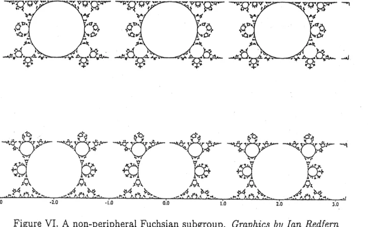
references as above.

Definition 2.4. We call a Fuchsian subgroup as in lemma 2.3 F-peripheral.

An example of

a

non-peripheral Fuchsian subgroup is shown in Figure

VI.

Question How

can

one

tell when

a

given Fuchsian subgroup is F-peripheral?

This is not

so

easy to answer;

a

large part of these lectures will involve in-vestigating exactly this point.

2.1

Special

Case

Example

Besides illustrating what is going on, the following example will

come

up

repreatedly and is essential to the proofof

some

of

our

main results.

Let $G=\langle AB\rangle\rangle$ be

a

once

punctured torus group. The complex distance $\delta(A, B)$ between $\mathrm{A}\mathrm{x}(A)$ and $\mathrm{A}\mathrm{x}(B)$ is given by;

$\sinh^{2}(\lambda_{A}/2)\sinh^{2}(\lambda_{B}/2)\sinh^{2}(\delta(A, B))=-1$.

Here $\lambda_{A}$ is the complex translation length of $A$ and TrA $=2\cosh(\lambda_{A}/2)$

.

The proof is an exercise with trace identities,

see

[PS95,

_{\S 2].}

1

Thus

Tr$\mathrm{A}$,Tr$B\in \mathbb{R}\Rightarrow-\sinh^{2}(\delta(A, B))>0$

which imples

In the first

case

Tr$A$, Tr$B$

are

coplanar and $G$ is Fuchsian (Why?); in the

second the

axes

do not meet but

are

perpendicular. In this

case

$G$ is

a

degenerate Schottky group obtained by identifying opposite circles

as

shown;

the four points of tangency lie

on a

rectangle. This is shown in Figure VII,

which shows a fundamental domain and how the limit set is formed in this

case.

Figure 7:

If $\partial C^{+}$ is pleated along $\mathrm{A}\mathrm{x}(A)$, then cutting $\partial C^{+}/G$ along the projection

of $\mathrm{A}\mathrm{x}(A)$,

we

obtain

a

punctured annulus. Lifting to

$\mathbb{H}^{3}$

we

get

a

piece

of plane with boundary

curves

Ax(A),

some

conjugate of $\mathrm{A}\mathrm{x}(A)$, and the

puncture; and similarly for $\partial C^{-}$ and _{$\mathrm{A}\mathrm{x}(B)$}. In fact

one can

show directly,

by studying fundamental domains for $G$ and how they

cover

$\Omega$, that in this

case

$\Gamma^{+}=\langle A, B^{-1}AB\rangle$ and $\Gamma^{-}=\langle B, A^{-1}BA\rangle$

are

$F$-peripheral. The details

Figure VI. A non-peripheral Fuchsian subgroup. Graphics by $Ian$

Redfern

This limit set corresponds to

a

surface group of genus 2.

Figure VII. Limit $\mathrm{s}\mathrm{e}_{1}\mathrm{t}$ for the special

case

example.

2.2

Real and

Complex

Fenchel

Nielsen

coordinates.

For the rest of this lecture,

we

shall discuss

a

more general way to

ensure

that

a

given Fuchsian subgroup is $F$-peripheral. First we need to recall

Fenchel-Nielsen and complex Fenchel-Nielsen coordinates for a

once

punctured torus.

These coordinates (for Teichm\"uller space and quasifuchsian space

respec-tively)

are

defined relative to

a

fixed generator pair $(U, V)$ corresponding to

geodesics $(\gamma, \delta)$

on

the torus $\Sigma$. For

more

detail

see

[KS97,

\S 4].

Figure 8:

The right side of figure 8 shows a punctured cylinder whose two boundary

curves

have equal lengths. This cylinder is shown lifted to $\mathbb{H}$ in figure 9. The

conjugate axes of $U$ and $V^{-1}UV$ project to the two boundary

curves

of the

cylinder and

are

identified by the transformation $V$, whose axis projects to

the curve $\delta$

on

$\Sigma$. Cutting the cylinder along the perpendiculars from the

cusp to the two boundary

curves

gives two pentagons with four right angles

and

one

cusp, which can be thought ofas two right angled hexagons with

one

degenerate side. From hyperbolic trigonometry, the length of the boundary

curve

$l_{\gamma}$ determines such a pentagon up to isometry. The two boundary

curves are

glued with a twist $t_{\gamma}\in \mathbb{R}$. To understand the twist better

we

lift

to $\mathbb{H}$; by definition

$t_{\gamma}$ is the signed distance $d(Y, V(X))$ as shown in figure 9.

Theorem 2.5. The Fenchel Nielsen coordinates $(l_{\gamma}, t_{\gamma})$ determine$\Sigma$ uniquely

up to conjugation in $\mathrm{P}\mathrm{S}\mathrm{L}(2, \mathbb{R})$.

ComplexF-N coordinates for quasifuchsian oncepunctured tori [Ta94], [Ko94],

[KS97], are made by exactly the

same

construction but with $\lambda_{\gamma}\in \mathbb{C}^{+}=$

$\{x+iy|x>0\}$ and $\tau_{\gamma}\in$ C. (Remember that Tr$g_{\gamma}=2\cosh(\lambda_{\gamma}/2).$) The

transformation $V$ glues $\mathrm{A}\mathrm{x}(V^{-1}UV)$ to $\mathrm{A}\mathrm{x}(U)$ with a shear of distance ${\rm Re}\tau_{\gamma}$

and

a

twist (bend) through angle ${\rm Im}\tau_{\gamma}$. Notice that the four endpoints of

the

axes

are in general not concyclic.

Exercise Prove that the endpoints of$\mathrm{A}\mathrm{x}(U),$ $\mathrm{A}\mathrm{x}(V^{-1}UV)$

are

concyclic iff

Figure 9:

Remark 2.6. Theorem 2.5 shows that for any $(\lambda_{\gamma}, \tau_{\gamma})\in \mathbb{R}^{+}\cross \mathbb{R}$,

we

can

write down generators $A,$ $B$ (or $U,$ $V$) for a group $G$ in which _{$[A, B]$} is

parabolic. Part of the content of theorem 2.5 is that this group is

auto-matically Fuchsian and represents a hyperbolic

once

punctured torus. In the

case

$(\lambda_{\gamma}, \tau_{\gamma})\in \mathbb{C}^{+}\cross \mathbb{C}$,

we can

still write down generators _{$A,$ $B$} (or _{$U,$ $V$}) for

the group $G$

.

However for general complex parameters, this group may be

neither free, discrete,

nor

quasifuchsian.

Complex Fenchel Nielsen Twists

or

Quakebends $([\mathrm{K}\mathrm{S}97, \S 5])$ For

$t\in \mathbb{R}$, the time $t$ F-N twist

or

earthquake $\mathcal{E}_{\gamma}(t)$ along

$\gamma$ is described in F-N

coordinates by $(l_{\gamma}, t_{\gamma})rightarrow(l_{\gamma}, t_{\gamma}+t)$. Likewise the time $\tau$ complex F-N twist

or

quakebend $Q_{\gamma}(\tau)$ is described in complex F-N coordinates

as

$(\lambda_{\gamma}, \tau_{\gamma})rightarrow$

$(\lambda_{\gamma}, \tau_{\gamma}+\tau),$ $\tau\in \mathbb{C}$

.

If _{${\rm Re}\tau=0$}, it is called

a

pure bend. In what follows,

we

shall be exploring exactly what happens to the

convex

hull when

we

perform

quakebends.

2.3

Developed

Surfaces

and

the Bending Away

Theo-rem

Part

1

In this section

we are

going to discuss the following$\mathrm{t}\mathrm{h}\mathrm{e}\mathrm{o}\mathrm{r},\mathrm{e}\mathrm{m}$, which is

a

slight

variant

on

[KS97, prop. 7.2].

Theorem 2.7 (Bending away theorem Part 1). Let $(l_{\gamma}, t_{\gamma})$ be the F-N

coordinates

_of

a Fuchsian

once

punctured torus group $G_{0}$

.

Then

for

small $\theta$, the groups with

complex F-N coordinates $(l_{\gamma}, t_{\gamma}+i\theta)$ are in $P_{\gamma}(i.e$. have

pleating locus $\gamma$

on

one or other side

of

To prove this theorem, we need to study the developed

_surface

associated

to

a

complex F-N twist.

The Developed Surface Say $\lambda_{\gamma}\in \mathbb{R}$

so

the endpoints of $\mathrm{A}\mathrm{x}(U)$ and

$\mathrm{A}\mathrm{x}(V^{-1}UV)$ are concyclic. The Nielsen region $N$ of $\Gamma=\langle U, V^{-1}UV\rangle$ maps

to

a

convex

part of

a

hyperbolic plane in $\mathbb{H}^{3}$

.

The image $V(N)$ lies in another

hyperbolic plane which meets $N$ along $\mathrm{A}\mathrm{x}(U)$ at an angle $\theta={\rm Im}\tau$. (This is

the “Micky Mouse example” of $[\mathrm{T}\mathrm{h}79,8.7.3].)$ The shaded region above the

hemisphere is $C$

.

Figure 10:

Continuing in this way, we get a map $\phi_{\tau}^{\gamma}=\phi_{\tau}$ : $(\mathrm{D}, G_{0})arrow(\mathbb{H}^{3}, G_{\tau})$

which conjugates the actions of$G_{0}=G(\lambda_{\gamma}, t_{\gamma})$

on

$\mathrm{D}$ with $G_{\tau}=G(\lambda_{\gamma}, t_{\gamma}+\tau)$

on $\phi_{\tau}^{\gamma}(\mathrm{D})\subset \mathbb{H}^{3}$ We call $\phi_{\tau}^{\gamma}$ the developed image of

$\mathrm{D}$ under the quakebend $Q_{\gamma}(\tau)$

.

Of course, for large $\theta={\rm Im}\tau$, we do not expect $\phi_{\tau}(\mathrm{D})$ to be embedded

in $\mathbb{H}^{3}$

.

Theorem 2.8. ($[\mathrm{K}\mathrm{S}97$, prop. 6.5]) In the situation

of

theorem 2.7, with

${\rm Re}\tau=0,$ ${\rm Im}\tau$ small, then $\phi_{\tau}^{\gamma}$ is an embedding which extends continuously to

a map $\partial \mathrm{D}arrow\partial \mathbb{H}^{3}$

.

The bending away theorem 2.7 is

a

corollary of 2.8 as follows:

(a) Show that $\phi_{\tau}(\mathrm{D})$ separates

$\mathbb{H}^{3}\cup\hat{\mathbb{C}}$

into two half spaces.

(b) Show that

one

of these half spaces is

convex.

(Note that this

uses

that

$\Sigma$ is a torus so that all bending is in the

same

direction.)

(c) Show that $\phi_{\tau}(\partial \mathrm{D})=\Lambda(G(\lambda_{\gamma}, t_{\gamma}+\tau))$ and that $\phi_{\tau}$ conjugates the actions

of $G_{0}$ and $G_{\tau}$

on

$\partial \mathrm{D},$ $\Lambda(G_{\tau})$ respectively.

(d) Conclude that $\phi_{\tau}(\mathrm{D})$ is a component of $\partial C_{0}(G_{\tau})$.

Proof of theorem 2.8. The idea is to

use

nested

cones

in $\mathbb{H}^{3}$. We write $C_{\delta}(\alpha, x)$ for the

cone

with vertex _$x$, angle $\alpha$, and central axis

$\delta$,

see

figure 11.

The key point in the proof is what we call the cone lemma [KS97, lemma

6.3].

Figure 11:

Suppose that $s\vdasharrow\eta(s)$ is

a

geodesic on $\Sigma$. As shown in figure 12 its

image under the developing map $\phi_{\tau}$ is a “bent” geodesic in $\mathbb{H}^{3}$

.

For a point

$\eta(s)$ on $\eta$, let $v(s)$ denote the

$\mathbb{P}$-geodesic based at the point _{$\phi_{\tau}(\eta(s))$} and

pointing in the forward direction along $\phi_{\tau}(\eta)$

.

If $\eta(s)$ is a bending point of $\phi_{\tau}(\eta)$, this doesn’t quite make

sense

since there

are

two forward directions of $\phi_{\tau}(\eta)$ corresponding to the directions immediately before and immediately

after the bend. For simplicity,

we

allow $v(s)$ to denote either. In all cases,

$C_{v(s)}(\alpha, \phi_{\tau}(\eta(s)))$ is

a cone

of angle $\alpha$ based at

a

point

on

$\phi_{\tau}(\eta)$ and pointing

in

one or

other of the forward directions along $\phi_{\tau}(\eta)$. The content ofthe

cone

lemma is that, provided

we

consider reasonably well spaced points along $\eta$,

these

cones are

nested. At bending points,

we

have two

cones

and the lemma

applies to them both.

Figure 12:

Theorem 2.9 (Cone Lemma). ($[\mathrm{K}\mathrm{S}97$, lemma 6.3])

Let $s\vdash\Rightarrow\eta(s)$ be a geodesic on $\Sigma_{f}$ and let $\alpha\in(0, \pi/2)$

.

Then there exist $\epsilon=\epsilon(\ell_{\gamma}, \alpha)>0$ and _{$d=d(\ell_{\gamma}, \alpha)>0$} such that

if

$Q_{\gamma}(i\theta)$ is a pure bend along

$C_{v(s)}(\alpha, \phi_{\tau}(\eta(s)))\supset c_{v(s+s’)(\alpha,\phi_{\tau}(\eta(s+s’)))}$

whenever $s’>d$.

We require the spacing condition $s’>d$ to take account of the two

cones

at the bending points. A

cone

obviously contains

cones

further out along

its own axis; the point is that hyperbolic geometry allows

us

the freedom to

make small bends.

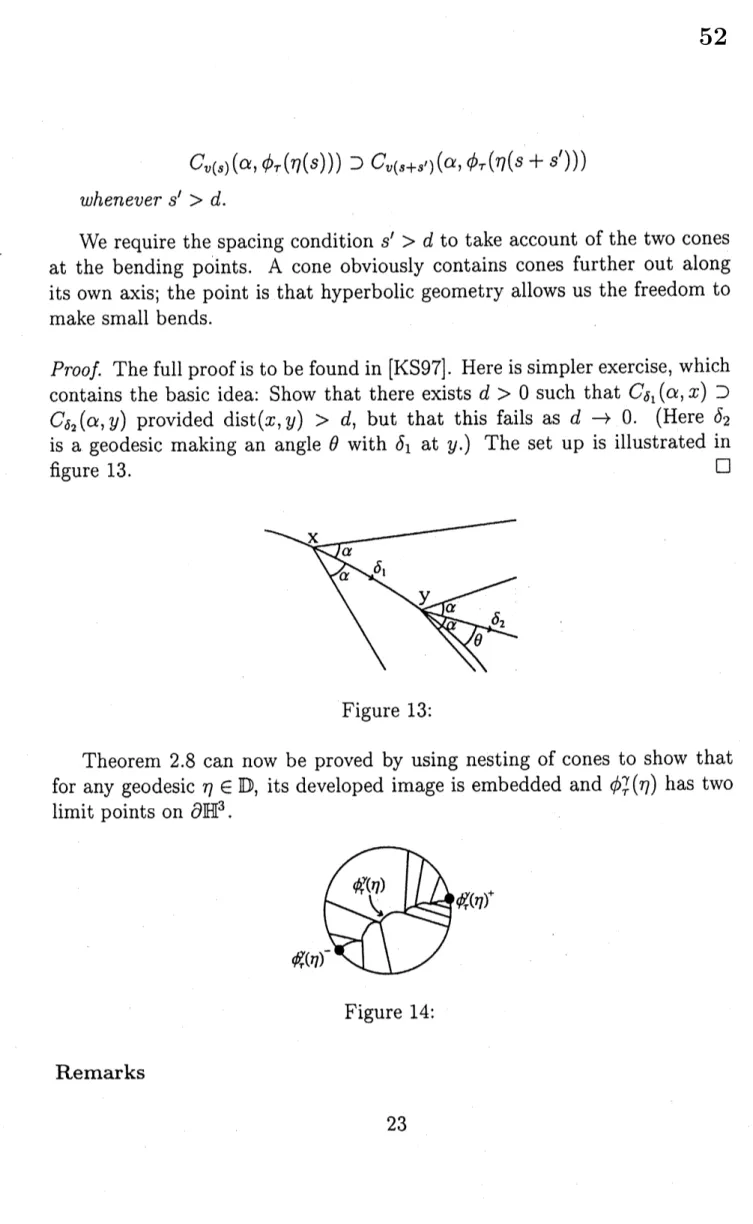
Proof.

The full proof is to be found in [KS97]. Here is simpler exercise, which

contains the basic idea: Show that there exists $d>0$ such that $C_{\delta_{1}}(\alpha, x)\supset$ $C_{\delta_{2}}(\alpha, y)$ provided dist$(x, y)>d$, but that this fails

as

$darrow \mathrm{O}$. (Here $\delta_{2}$

is a geodesic making an angle $\theta$ with $\delta_{1}$ at _$y.$) The set up is illustrated in

figure 13. $\square$

Figure 13:

Theorem 2.8

can now

be proved by using nesting of

cones

to show that

for any geodesic $\eta\in \mathrm{D}$, its developed image is embedded and $\phi_{\tau}^{\gamma}(\eta)$ has two

limit points

on

$\partial \mathbb{H}^{3}$.

Figure 14:

(a) The proofof theorem 2.7 has been done for

a

pure bend $({\rm Re}\tau=0)$ but

we

can

extend to general $\tau$ by first doing

an

earthquake (F-N twist) by ${\rm Re}\tau$ in $\mathrm{D}$ along

$\gamma$

.

It would also be possible to give a direct proof.

(b) The

same

proof will clearly work

more

generally starting at

some

group

$G\in P_{\gamma}$ and bending

a

small amount

on

$\gamma$.

(c) Another proofof (b)

can

be given

more

elementary means, by showing

that peripheral circles persist under small deformations. This

was

done

in [KS93] and [KS94]. We need the ideas in the above proof later.

(d) Note the difficulty of extending to genus greater than 1. If

we

want to bend away from $F$ along two disjoint simple closed

curves

simultane-ously,

we

must

ensure

the bending angle is in the

same

direction along

both, otherwise

we

loose convexity.

2.4

Controlling

the pleating locus

on

both sides.

The bending away theorem 2.7 controls the pleating locus of one side, say

$p\ell^{+}$ on $\partial C^{+}$. (Which side is which depends on which way we bend.)

Now

we want to simultaneously control $p\ell^{-}$ Suppose $\gamma’\in S(\Sigma)$ and we want

$p\ell^{-}=\gamma’$

.

A necessary condition is that Tr$\gamma’\in \mathbb{R}$. How can this be achieved

near

Fuchsian space $F$?

To

answer

this question,

we

make use of the fact that Tr$\gamma’$ is

holomor-phic

on

$QF$ and real valued

on

$F$

.

In particular, it is holomorphic

on

the

quakebend plane

$Q_{\gamma}(\tau)=$

{

$G(\lambda_{\gamma},$ $\tau)|\lambda_{\gamma}$ fixed, $\tau\in \mathbb{C}$

}.

Notice that $Q_{\gamma}(\tau)\cap F=\mathcal{E}_{\gamma}(t)$is exactlythe earthquake line_$\tau=t,$$t\in \mathbb{R}$. Now

the real locus of

a

holomorphic function has

a

very special form: figure 15

illustrates the real locus of

a

holomorphic function $f$ which is real

on

the real

axis in the $\tau$-plane. The only branching

can

be at

a

critical point of _$f$.

Now

we use a

famous result due to Kerckhoff and Wolpert,

see

[Ke83]

and [Wo82].

Theorem 2.10. On $\mathcal{E}_{\gamma}(t)f\lambda_{\gamma’}=\lambda_{\gamma’}(t_{\gamma})$ has $a$ unique critical point$t_{\gamma}^{0}$ which is a minimum; in addition $\lambda_{\gamma}’’,(t_{\gamma}^{0})>0$

.

Figure 15:

This allows us to deduce exactly how the pleating variety $P_{\gamma,\gamma’}$ meets

Fuchsian space $F$

.

On a fixed quakebend plane, $l_{\gamma}$ has a fixed length which

we

denote by $c$. We denote this by writing $Q_{\gamma}^{c}(\tau)$, and

we

denote by$p(\gamma, \gamma’, c)$

the critical point $t_{\gamma}^{0}$. Here $l_{\gamma’}$ is minimal on the $\gamma$-earthquake path $\mathcal{E}_{\gamma}=$

$\mathcal{E}_{\gamma}^{\mathrm{c}}$. It follows from the antisymmetry of the derivative $dl_{\mu}/d\tau_{\nu}=-dl_{\nu}/d\tau_{\mu}$ that $p(\gamma, \gamma’, c)$ is also the minimum of $l_{\gamma}$ on the $\gamma’$-earthquake path through

$p(\gamma, \gamma’, c)$. (We are disguising in this

some

facts which are fairly easy to

deduce from Kerckhoff’s theorem 2.10, in particular that for a given $\gamma,$ $c$

there is a unique earthquake path

on

which $l_{\gamma}=c$. We shall

come

back to

this in more detail in lecture 6, see also [KS98,

\S 6].)

Theorem 2.11 (Bending Away Theorem Part 2). ($[\mathrm{K}\mathrm{S}98$, theorem 8.9])

In $Q_{\gamma}^{c}(\tau),$ $P_{\gamma,\gamma’}$ meets $F$ exactly in the

Kerckhoff

critical point $p(\gamma, \gamma^{l}, c)$.

Proof.

Let $\delta’$ be a complementary generator to $\gamma’$

.

Since Tr$\gamma’\in \mathbb{R}$

we

can

make the complex F-N construction relative to $(\gamma’, \delta’)$ and obtain adeveloped

surface $\phi_{\tau}^{\gamma’},(\mathrm{D})$ bent along $\gamma’$ by an angle ${\rm Im}\tau’$. Since ${\rm Im}\tau’=0$

on

$F$, and

since $\tau’$ is

a

continuous function of

$\tau=\tau_{\gamma}$, we

see

that near $F,$

${\rm Im}\tau’$ is small

and the same proof as before shows that $\phi_{\tau}^{\gamma’},(\mathrm{D})$ is a

$\mathrm{c}\mathrm{o}$

,mponent

of

$\partial C$. $\square$

Corollary 2.12. ($[\mathrm{K}\mathrm{S}97$, theorem 3.2]) Suppose that $\gamma,$ $\gamma’\in S(\Sigma),$ $\gamma\neq\gamma^{J}$.

Then $P_{\gamma,\gamma’}\neq\emptyset$

.

Exercise What is wrong with the above argument when $\gamma=\gamma’$?

Example 2.13. Suppose that $A,$$B$ are generators of$G$ (aquasifuchsian

once

punctured torus group) and

we

want to find groups such that $|p\ell^{+}|=\mathrm{A}\mathrm{x}(A)$,

$|p\ell^{-}|=\mathrm{A}\mathrm{x}(B)$. In this special

case

there is an explicit formula which relates

the traces and the twists:

(This is proved in [PS95]; it

can

be checked by differentiating using Kerck-hoff’s formula $\frac{d}{d}\lambda\ovalbox{\tt\small REJECT}\lambda_{A}=-\cosh(\delta(A, B)).)$ So $\lambda_{A},$$\tau_{B}\in \mathbb{R}$ implies that either

${\rm Im}\tau_{A}=0$, in which

case

$G$ is Fuchsian, or that ${\rm Re}\tau_{A}=0$ in which

case

we

have a pure bend. This is our special case example 2.1.

Lecture 3: Irrational measured laminations

and Complex Length.

Statements of the

main

technical

results.

Irrational laminations can be viewed as a completion

_of

the space $S(\Sigma)$

of

simple

closed curves on a hyperbolic

_surface

$\Sigma$. When $\Sigma$ is a punctured torus, they can

be thought

_of

as

_families

_of

lines

_of

irrational slopes in the plane. In this lecture,

we discuss how some key concepts extend to this case and then introduce the main

technical results we shall need. Sections 3.1 to 3.6 apply to general hyperbolic

surfaces

$\Sigma$ unless otherwise stated.

3.1

Geodesic

Laminations

Good references for this section

are

[EM87] and [CEG87].

Definitions A geodesic lamination

on

ahyperbolic surface $\Sigma$ is aclosed set

which is

a

union ofpairwise disjoint simple (not necessarily closed) geodesics.

A geodesic lamination is measured if it carries a transverse

measure

$\nu$. This

means there is

a

measure

$\nu_{T}$ on each transversal $T$ to $\nu$ which is invariant

under the push-forward maps along leaves, as illustrated in figure 16.

$v(\mathrm{T}_{1})=v(\mathrm{T}_{2})$

$v(\mathrm{T}_{5})=v(\mathrm{T}_{3})+v(\mathrm{T}_{4})$

Figure 16:

$\underline{\mathrm{E}\mathrm{x}\mathrm{a}\mathrm{m}\mathrm{p}\mathrm{l}\mathrm{e}}$ Let $\gamma\in S(\Sigma)$ be a simple closed loop. Then $\gamma$ is a geodesic

lamination which always carries the transverse

measure

$\nu=c\delta_{\gamma},$ $c>0$ where

Notation Here is

some

notation which

we

shall

use:

$\mathcal{G}\mathcal{L}(\Sigma)$ $=$

{geodesic

laminations

on

$\Sigma$

}

$\lambda 4\mathcal{L}(\Sigma)$ $=$

{measured

geodesic laminations on $\Sigma$

}

At$\mathcal{L}_{\mathbb{Q}}(\Sigma)$ $=$ $\{c\delta_{\gamma}|\gamma\in S(\Sigma)\}$

Thus $\mathcal{M}\mathcal{L}_{\mathbb{Q}}(\Sigma)$ is the set of rational measured laminations

on

$\Sigma$. Notice that $\mathbb{R}^{+}$ acts

on

$\mathcal{M}\mathcal{L}(\Sigma)$ by $t,$ $\nurightarrow t\nu$ where $(t\nu)(T)=t\nu(T),$ $T$ a transversal. We

define

$P\mathcal{M}\mathcal{L}(\Sigma)=$ {projective measured laminations on $\Sigma$

}

$=\mathcal{M}\mathcal{L}(\Sigma)/\mathbb{R}^{+}$

For $\nu\in \mathcal{M}\mathcal{L}(\Sigma)$,

we

write $[\nu]$ for its projective class in $P\mathcal{M}\mathcal{L}$, and $|\nu|$ for its

support in $\mathcal{G}\mathcal{L}$.

WARNING Not all geodesic laminations

are

measured! A geodesic

spiralling into a closed geodesic cannot support a transverse

measure-

the

measure

of transversal

near

the limit geodesic would be infinite. This is

shown in figure 17.

Figure 17:

3.2

Topologies

on

$\mathcal{G}\mathcal{L}$

and

a

$\mathcal{L}$

.

There

are

two topologies which

are

commonly used:

Geometric topology on $\mathcal{G}\mathcal{L}$

.

In this topology, laminations $L_{1},$ $L_{2}\in \mathcal{G}\mathcal{L}$

are

close if every point in $L_{1}$ is close to a point in $L_{2}$ and vice

versa.

Since geodesics diverge, this

means

tangent directions

are

close.

Measure topology$\mathcal{M}\mathcal{L}\mathrm{o}\mathrm{n}\mathcal{M}\mathcal{L}$

.

This is the weak topology of

measures on

Figure 18:

WARNING These topologies

are

not the same!! For example, $\delta_{\gamma}$ and

$100\delta_{\gamma}$

are

close in $\mathcal{G}\mathcal{L}$ but not in $\mathcal{M}\mathcal{L}$

.

A

more

subtle example is shown in figure 18. Take

a

sequence of closed

geodesics $(\gamma_{n})$ of which

some

parts

are

far from

$\gamma$, but which also spiral $n$

times around $\gamma$. Then

$\frac{1}{n}\delta_{\gamma_{n}}\mathcal{M}\mathcal{L}\prec\delta_{\gamma}$ but

$| \frac{1}{n}\delta_{\gamma_{n}}|=\gamma_{n}$ is far from $\gamma$ in $\mathcal{G}\mathcal{L}$.

A lamination $L$ may carry several different projective

measure

classes,

so we

can

have laminations equal in $\mathcal{G}\mathcal{L}$ and but different in $P\mathcal{M}\mathcal{L}$. This

does not happen on the punctured torus because of the property of unique

ergodicity:

a

(measurable) lamination $L$ is uniquely ergodic if it carries a

unique projective measure class. In this case, up to a constant multiple,

$\nu(T)=\lim_{narrow\infty}i(l_{n}, T))/n$ where $l$ is any leaf of $L$ and $l_{n}$ is an arc of $l$ of

length $n$ from some fixed initial point. On a general surface, the property

of unique ergodicity is generic. However, it is special to the punctured torus

(and four holed sphere) that it holds for every $L\in \mathcal{M}\mathcal{L}$.

On the torus, the followinglemmarestricts the bad examples which

occur.

Lemma 3.1 (Convergence Lemma). ( $[\mathrm{K}\mathrm{S}98$, lemma 2.1]) Let $\Sigma$ be a

once

punctured torus and let $\nu_{0}\in \mathcal{M}\mathcal{L}-\mathcal{M}\mathcal{L}_{\mathbb{Q}}$.

If

$\nu$ is close to $\nu_{0}$ in $\mathcal{M}\mathcal{L}$,

then $|\nu|$ is close to $|\nu_{0}|$ in $\mathcal{G}\mathcal{L}$

.

Remark We need the condition $\nu_{0}\not\in \mathcal{M}\mathcal{L}_{\mathbb{Q}}$ because of the situation shown

in figure 19, in which $\frac{1}{n}\delta_{A^{n}B}arrow\delta_{A}\mathcal{M}\mathcal{L}$ but $|\delta_{A^{n}B}|\underline{\mathcal{G}}\mathcal{L}\neq+|\delta_{A}|$.

Figure 19:

In the

case

of a surface of higher genus the geodesic $A$ of the above

example

can

be replaced by

an

irrational lamination. This explains why in

Proof.

First, suppose that $\nu$ is close to $\nu_{0}$ in

$\mathcal{M}\mathcal{L}$

.

The lamination $|\nu_{0}|$

can

be covered by “flow boxes”

as

shown in figure 20. The “horizontal” sides

are

short and the “vertical” sides

are

long. Notice $|\nu_{0}|$ has

no

“horizontal”

arcs.

We claim that if $\nu$ is close enough to $\nu_{0}$, the

same

is also true of $|\nu|$.

Figure 20:

The proofis by considering the

measures

of transversals: clearly,

as

shown

in figure 21, $x+y\sim t,$ $x+z+w\sim 0,$ $w+v\sim t,$ $y+z+v\sim \mathrm{O},$ $x,$ $y,$ $z,$ $w,$ $t\geq 0$

$\Rightarrow z=0$. So $|\nu|$ has a “vertical leaf’ close to $|\nu_{0}|$.

This part of the proof works in any

genus.

Figure 21:

Now for the

converse.

We need to show that there

are

leaves of $|\nu_{0}|$

near

any long arc of $|\nu|$

.

If not, we can

$\mathrm{t}\mathrm{a}_{\mathcal{M}L}\mathrm{k}\mathrm{e}\mathrm{a}$ limit and find

a

leaf

$l\not\in|\nu_{0}|$ which

is

a

limit of leaves of $|\nu_{n}|$ where _{$\nu_{n}arrow\nu_{0}$}. If $l\cap|\nu_{0}|=\emptyset$, then

we

get the

pictures shown in figure 22. The picture

on

the left shows the punctured

bigon obtained by cutting $\Sigma$ along the two boundary leaves of $|\nu_{0}|$. (This is

where

we use

the hypothesis $\nu_{0}\not\in \mathcal{M}\mathcal{L}_{\mathbb{Q}}.$) The leaf$l$ has

no

choice but to

run

from one ideal vertex of this bigon to itself.

Now cut the torus along any simple closed

curve

which meets $l$. The

result is shown in on the right hand side of figure 22. Any lamination in $\mathrm{A}4\mathcal{L}$

would give equal weight to the inner and outer boundaries of the resulting

punctured annulus $A$. On the other hand,

one

sees

from the figure that the

Figure 22:

isimpossible to approximate any possible

non zero

weight

on

$l$ by laminations

in $\mathcal{M}\mathcal{L}$

.

For

more

details,

see

[Th79, 9.5.2].

We may therefore

assume

that $l\cap|\nu_{0}|-\neq\emptyset$, which

means we

can

find

a

flow box for $|\nu_{0}|$ in which $l$ is

a

$‘(\mathrm{h}\mathrm{o}\mathrm{r}\mathrm{i}\mathrm{z}\mathrm{o}\mathrm{n}\mathrm{t}\mathrm{a}\mathrm{l}$”

arc.

This is also impossible by

the first part of the proof. $\square$

3.3

The Thurston

Picture

of

$P\mathcal{M}\mathcal{L}$

In general, $P\mathcal{M}\mathcal{L}(\Sigma)$ is a sphere (of dimension $6g-7$ for a closed surface

$\Sigma$ ofgenus

$g$). This sphere compactifies the Teichm\"uller space $\mathcal{T}(\Sigma)$, which

is a ball of dimension $6g-6$

.

Roughly, (this is not the actual definition),

$\xi_{n}\in \mathcal{T}(\Sigma)arrow[\delta_{\gamma}]\in P\mathcal{M}\mathcal{L}$ if $\xi_{n}arrow\partial \mathcal{T}$ and $l_{\gamma}(\xi_{n})$ is bounded. In the

torus

case

the picture

was

shown in figure 1. The set ofirrational projective

measured laminations is identified with $\mathbb{R}\cup\{\infty\}-\mathbb{Q}$,

so

that $P\mathcal{M}\mathcal{L}=S^{1}$.

This fits with Wright’s enumeration of $S(\Sigma)$

as

explained in lecture 1.

3.4

The

Bending

Measure

on

$\partial C$

and

the Continuity

Theorems

Definition 3.2. ([EM87], [CEG87]) Let $\Sigma$ be a hyperbolic surface, $\Gamma$ a

Fuchsian group with $\Sigma=\mathbb{H}/\Gamma,$ $G$

a

Kleinian group. A pleaied

surface

is

a

map $\sigma$ :

$\mathbb{H}^{2}arrow \mathbb{H}^{3}$ (or

$\Sigmaarrow \mathbb{H}^{3}/G$) such that:

(a) $\mathbb{H}^{3}\sigma \mathrm{i}\mathrm{s}$

.

an isometry from

$\mathbb{H}$ to its image with the path metric induced from

(b) $\sigma_{*}:$ $\pi_{1}(\Sigma)=\Gammaarrow G$ is

an

injection.

(c) For each $x\in\Sigma$, there exists at least

one

geodesic $\gamma$ containing $x$ such

that $\sigma|_{\gamma}$ is an isometry.

The bending locus is the set of geodesics in $\mathbb{H}$ through which there is

on

$\Sigma$, denoted by _$B(\sigma)$

.

In general, the image $\sigma(\mathbb{H})$ is neither

convex

nor

embedded in $\mathbb{H}^{3}$

.

Definition 3.3. A lamination $L\in \mathcal{G}\mathcal{L}(\Sigma)$ is realized in $\mathbb{H}^{3}/G$

if

there is a

pleated

_surface

$\sigma$ : $\Sigmaarrow \mathbb{H}^{3}/G$ with $L\subset B(\sigma)$.

In this definition, the hyperbolic structure on $\Sigma$ is left unspecified, to be

determined by the map and the structure

on

$\mathbb{H}^{3}$.

Theorem 3.4. ([Th79], [CEG87]) Let $G$ be quasifuchsian and$L\in \mathcal{G}\mathcal{L}(\Sigma)$.

Then $L$ is realized in $\mathbb{H}^{3}/G$

.

Proof.

The idea is to make a direct (quite easy) construction if $L$ has only

finitely many leaves and then

use

“compactness of pleated surfaces” to take

limits. It is explained in detail in [CEG87, chapter 5]. $\square$

3.5

The Convex

$\mathrm{H}\mathrm{u}\mathrm{l}\mathrm{l}$

Boundary

Theorem 3.5. (Thurston, [EM87] Chapter 1) Let $G$ be a finitely generated

Kleinian group and let $\partial C_{0}$ be a component

of

$\partial C$, the convex hull boundary

of

$\mathbb{H}^{3}/G$

.

Then $\partial C_{0}$ carries an intrinsic hyperbolic metric induced

from

the

metric $\mathbb{H}^{3}$, making it a pleated

surface.

The bending $lam\dot{\iota}nation$ carries a

natural transverse measure, the bending

measure

$pl(\partial C_{0})\in \mathcal{M}\mathcal{L}(\partial C_{0}/G)$.

Remark It is clear that in addition, $\partial C_{0}$ is

convex

(i.e. cuts off a

convex

half space) and embedded.

The idea for constructing the bending

measure

is illustrated in figure 23

A support plane is a half space touching $\partial C$ with $C$ entirely on

one

side. The

Figure 23:

figure 23 shows a collection ofsupport planes forming a “roof”

over

$C$;

ofa transversal $T$ is defined by $pP(T)= \inf\sum\theta_{i},\mathrm{w}\mathrm{h}\mathrm{e}\mathrm{r}\mathrm{e}$ the infimum is taken

over

all possible families of support planes sitting “over’) _{the transversal} $\mathrm{T}$,

which joins $x$ to $y$ in the figure. Distance

on

$\partial C$

can

be defined in a similar

way. We call the induced hyperbolic metric on $\partial C_{0}$, the

flat

structure $F(\partial C_{0})$

of$\partial C_{0}$.

Theorem 3.6 (The continuity theorem). [KS95] Let $\xirightarrow G_{\xi}$ be a

holo-morphic family

_of

Kleinian groups. Then

_for

a

_fixed

component $\partial C_{0}$, the

maps $\xi-*p\ell(\xi)\in \mathcal{M}\mathcal{L}$ and $\xirightarrow F(\partial C_{0}(\xi))\in \mathcal{T}(\Sigma)$

are

continuous.

Proof.

There is aretraction map $r$ : $\Omegaarrow\partial C$ which maps $z\in\Omega$ to the nearest

point on $\partial C$,

seen

by drawing expanding horoballs at

$z$

as

in figure 24.

Figure 24:

This also defines a support plane at $r(z)$

.

We study the continuity of

the map $\hat{r}$ : _{$\Omega\cross \mathrm{D}\mathrm{e}\mathrm{f}arrow Z(\partial C)$} where _{$Z(\partial C)$} is the set of support planes to

$\partial C$ with the obvious topology. One shows that $\hat{r}$ is uniformly continuous

on

compact subsets of $\Omega\cross \mathrm{D}\mathrm{e}\mathrm{f}$

so

that any approximating rooffor

one

group is

close to

a

roof for a nearby group. It follows that the bending

measure

and

flat metrics are also close. $\square$

3.6

Length and Complex Length

Length of a measured lamination

on

a hyperbolic surface $\Sigma$ If

$\gamma\in S(\Sigma)$, then its hyperbolic length $l(\gamma)$ is given by Tr$\gamma=2\cosh(l(\gamma)/2)$. If $c\delta_{\gamma}\in \mathrm{A}4\mathcal{L}_{\mathbb{Q}}(\Sigma)$, set 1$(c\delta_{\gamma})=cl(\gamma)$. We want to extend this to $l:\mathcal{M}\mathcal{L}(\Sigma)arrow$ $\mathbb{R}^{+}$. One way

is to

cover

$|\nu|,$ $\nu\in \mathrm{A}4\mathcal{L}$, by flow boxes $B_{i}$ and integrate:

$l( \nu)=\sum_{i}\int_{T_{i}}t(L_{x}\cap B_{i})d\nu_{T_{\mathfrak{i}}}(x)$, where $L_{x}$ is the leaf of $|\nu|$ through $x$ in the

transversal $T_{i}$

.

Theorem 3.7. ([Ke83], [Ke85])

_If

$\nu_{n}\in \mathcal{M}\mathcal{L}_{\mathbb{Q}\mathrm{z}}\nu_{n}\mathcal{M}\mathcal{L}arrow\nu,$ _{$\xi\in \mathcal{T}(\Sigma)$}, then $(l_{\nu_{n}}(\xi))$ has a unique limit $l_{\nu}(\xi)$. The convergence is

uniform

on

compact

subsets

_of

$\mathcal{T}(\Sigma)$

.

Complex length of a loxodromic. If $g\in \mathrm{S}\mathrm{L}(2, \mathbb{C})$ then its complex

length $\lambda_{g}$ is given by Tr$g=2\cosh(\lambda_{g}/2)$

.

Here $\lambda_{g}=l_{g}+i\theta_{g}$ where $l_{\mathit{9}}$ is the

translation length along the axis and $\theta_{g}$ is the twist.

Note There is

a

major difficulty in extending this definition to $\mathcal{M}\mathcal{L}_{\mathbb{Q}}$ since $\theta_{g}$ is only defined mod $2\pi$

.

One possible solution is explained next.

Complex length of a measured lamination. We want to extend the

length function $l_{\nu}$ from $\mathcal{T}(\Sigma)$ to $QF(\Sigma)$. We have $F(\Sigma)=\mathcal{T}(\Sigma)\mapsto QF(\Sigma)$.

For $\gamma\in S(\Sigma)$, choose the branch of$\lambda_{g}=\lambda_{g}(\xi),$ $g=g(\gamma)$, which is real valued

on

$F$

.

Then define $\lambda_{c\delta_{\gamma}}=c\lambda_{g(\gamma)}$. Notice that this choice of

a

specific branch

gets

us

round the difficulty ofdefining $c\theta_{g}$ mod $2\pi$

Consider the family of functions $\lambda_{\mathrm{c}\delta_{\gamma}}$ : $QFarrow \mathbb{C}$. These are holomorphic

and avoid the negative half plane $\mathbb{C}^{-}=\{z\in \mathbb{C}|{\rm Re} z<0\}$. Hence they

are

a normal family,

see

for example [Be91, theorem 3.3.5]. So if $\nu_{n}\prec\nu \mathcal{M}\mathcal{L},$

$\nu_{n}\in$ $\mathcal{M}\mathcal{L}_{\mathbb{Q}}$, then $(\lambda_{\nu_{n}})$ has a convergent subsequence. By Kerckhoff’s theorem, $(\lambda_{\nu_{n}})$ has a unique limit

on

$F$ and hence (holomorphic functions!) on $QF$.

Moreover $\lambda_{\nu}$ is non-constant since it is non-constant

on

$F$ by Kerckhoff. This

defines complex length.

Note $\mathrm{A}t\mathcal{L}\mathrm{E}\mathrm{q}\mathrm{u}\mathrm{i}\mathrm{c}\mathrm{o}\mathrm{n}\mathrm{t}\mathrm{i}\mathrm{n}\mathrm{u}\mathrm{i}\mathrm{t}\mathrm{y}$

means we

can

take diagonal limits:

$\xi_{n}arrow\xi\in QF$

and $\nu_{n}arrow\nu$ implies $\lambda_{\nu_{n}}(\xi_{n})arrow\lambda_{\nu}(\xi)$

.

3.7

Statement of Main Technical Results

We

can

now

state the main technical results

we

shall need. From now on,

$G$ is

a

quasifuchsian

once

punctured torus group, $p^{p+}$ and $pP^{-}$ the bending

measures

on

$\partial C^{+}/G$ and $\partial C^{-}/G$. For $\mu,$ $\nu\in A4\mathcal{L}$, set

$P_{[\mu],[\nu]}:=\{\xi\in QF|[p\ell^{+}]=[\mu], [p\ell^{-}]=[\nu]\}$.

(Often

we

shall be sloppy and write $P_{\mu,\nu}$ for $P_{[\mu],[\nu]}.$) Also

we

write

$P_{\mu}=P_{[\mu]}=$

{

$\xi\in QF|[p^{p+}]=[\mu]$

or

$[p\ell^{-}]=[\mu]$

}.

Theorem 3.8 (Real Length Lemma). ($[\mathrm{K}\mathrm{S}98\mathrm{a}$, theorem 6.5]) Suppose

that $\xi\in QF,$$\xi\in P_{\mu}$. Then $\lambda_{\mu}(\xi)\in \mathbb{R}$.

The idea of the proof is obviously to take limits, but we need

care

to

ensure

that $\lambda_{\mu}(\xi)\in \mathbb{R}$ is impossible

on

open sets in $QF$

.

The proof is given

in lecture 5.

Theorem 3.9 (Local Pleating Theorem, Version 1). ([$\mathrm{K}\mathrm{S}98$, theorem

8.6]) Suppose $\nu_{0}\in \mathcal{M}\mathcal{L}-\mathcal{M}\mathcal{L}_{\mathbb{Q}_{J}}\xi_{0}\in P_{\nu_{0}}\cup F$. Then there are neighbourhoods

$U$

of

$\xi_{0}$ in $QF$ and $W$

of

$[\nu_{0}]\in P\mathrm{A}4\mathcal{L}$ such that $[\delta_{\gamma}]\in W\cap P\mathcal{M}\mathcal{L}_{\mathbb{Q}\mathrm{z}}\xi\in U$,

$\lambda_{\gamma}(\xi)\in \mathbb{R}$ implies _{$\xi\in P_{\gamma}\cup F$}.

Theorem 3.10 (Local Pleating $\mathrm{T}\mathrm{h}‘ \mathrm{e}\mathrm{o}\mathrm{r}\mathrm{e}\mathrm{m}$, Version 2). ([

$\mathrm{K}\mathrm{S}98$, theorem

8.1])

Suppose $\nu_{0}\in \mathcal{M}\mathcal{L}_{f}\xi_{0}\in P_{\nu_{0}}\cup F$. Then there is a neighbourhood $U$

of

$\xi_{0}$

in $QF$ such that $\xi\in U,$ $\lambda_{\nu_{0}}(\xi)\in \mathbb{R}$ implies $\xi\in P_{\nu_{0}}\cup F$.

Remarks on theorems 3.9 and 3.10. One should compare theorem 3.9

to the theory oflocal deformations for cone manifolds. (But notice it applies

equally to irrational laminationsand also that

we

do not need to

assume

there is a continuous path of deformations from $\xi_{0}$ to $\xi.$) It would be tempting to

combine 3.9 and 3.10 and allow $\nu$ to vary in

a

neighbourhood of $\nu_{0}$ in 3.10.

However this result would be false in higher genus: take

a

surface of genus

two and disjoint loops $\gamma$ and $\gamma’$

.

Bending away from $F$ in opposite directions

along the two curves, we find $\frac{1}{n}\delta_{\gamma’}+\delta_{\gamma}arrow\delta_{\gamma},$$\lambda_{\gamma’}(\xi)\mathcal{M}\mathcal{L}\in \mathbb{R}$ but $\xi\not\in P_{\gamma’}$.

Figure 25:

For the special

case

of

a

torus, the result is true since there is

a

maximum

of

one

bending angle $($uniquely $\mathrm{e}\mathrm{r}\mathrm{g}\mathrm{o}\mathrm{d}\mathrm{i}\mathrm{c}\mathrm{i}\mathrm{t}\mathrm{y})^{\backslash }$

.

The proof is

more

complicated

and not needed

so

omitted here.

Theorem 3.11 (Limit Pleating Theorem). ($[\mathrm{K}\mathrm{S}98\mathrm{a}$, theorem 5.1])

Sup-pose $\mu,$ $\nu\in \mathcal{M}\mathcal{L},$ $[\mu]\neq[\nu]$. (Equivalently, on the punctured torus, using