ON
THE
CONFLUENT HYPERGEOMETRIC
FUNCTIONS
IN
2
VARIABLES
YONGYAN LU (陸永岩)
Graduate School
of
Mathematical SciencesThe University
of
Tokyo\S 0.
Introduction.Let $M(r, n)$ be the set of complex matrices, $\lambda=(\lambda_{0,\ldots,l-1}\lambda)$ apartition of
$n$. We conside the action of$GL(\Gamma, \mathbb{C})\cross H_{\lambda}$ on $Z_{r,n}:=\{z\in M(r, n)$
:
rankz $=$$r\}$ defined by
$GL(r, \mathbb{C})\cross Z_{r,n}\cross H_{\lambda}arrow Z_{r,n}$
$(^{*})$
$(g, z, h)$ $\mapsto gzh,$
.
where $H_{\lambda}=J(\lambda_{0})\cross\cdots\cross J(\lambda_{l-}1)\subset GL(n)$ be the associated maximal abelian
subgroup withrespect to $\lambda^{\mathrm{c}},$
$J(m)= \{\sum_{i=0}^{m1}hi\Lambda i$ : $h_{0}\in \mathbb{C}_{}^{\cross},$$h_{1,\ldots,m-1}h\in \mathbb{C}\}$
$]$ A $:=(_{0}^{0}$ $.01.$
.
$\cdot...c\dagger \mathit{4}.$ . $0_{1}0)$ Let $\iota$ :$H_{\lambda} arrow\prod_{:}(\mathbb{C}^{\cross}\cross \mathbb{C}^{\lambda.-1})$. For $z\in Z_{r,n}$, the generalized confluent
hypergeometric function (CHG function, for short) is defined as
(0.1) $\Phi(z;\alpha)=\int_{\Delta}\chi(\iota^{-1}(tZ);\alpha)\cdot\omega$
where $\alpha$ be an $n$-tuple of complex numbers satisfying $\sum_{i=}^{l-1}0\alpha^{(}0i$
)
$=-\Gamma,$ $\lambda$ the
$t$-space depending on$z$and$\alpha$. The function$\Phi$ admitsthefollowing symmetries:
(0.2) $\Phi(gz;\alpha)=(\det g)-1\Phi(z;\alpha)$ $g\in GL(r, \mathbb{C})$
(0.3) $\Phi(zh_{\lambda;\alpha})=\chi(h_{\lambda})\Phi(z;\alpha)$ $h_{\lambda}\in H_{\lambda}$
.
(0.4) $\Phi(zw_{\lambda^{4}}, \alpha)=\Phi(z;\alpha^{t}w_{\lambda})$ $w_{\lambda}\in W_{\lambda}$,
where $W_{\lambda}$ is an analogue of the Weyl group, see [K-K] and Section 1.
The CHG functions $\Phi$ on $Z_{2,4}$ and $Z_{2,5}$ for various partitions $\lambda$ of 4 and
5 were investigated in the papers $[\mathrm{K}- \mathrm{H}-\mathrm{T}],[\mathrm{O}- \mathrm{K}]$ and [K-K]. It is known that
the functions $\Phi$ are generalizations of Gauss’, Kummer’s, Bessel’s, Hermite’s,
Airy’s functions and the classical hypergeometric functions of two variables,
i.e., $F_{1},$$\phi_{1},$$\phi_{2},$$\phi_{3},$$G_{2},$$\Gamma_{1,2}\Gamma$ in Horn’s list $([\mathrm{E}\mathrm{r}\mathrm{d}1])$
.
In this talk, we study thehypergeometric functions of type $\lambda$ in two variables on the strata of the set
$M(3,6)$ of$3\cross 6$ complex matrices
\S 1.
Construction of the group $W_{\lambda}$.
Set $\lambda^{(0)}=(1,1,1,1,1,1),$ $\lambda^{(1)}=(2,1,1,1,1),$ $\lambda^{(2)}=(2,2,1,1),$ $\lambda^{(3)}=$ $(2,2,2),$ $\lambda^{(4)}=(3,1,1,1),$ $\lambda^{(5)}=(3,2,1),$ $\lambda^{(6)}=(3,3),$ $\lambda^{(7)}=(4,1,1)$ and
$\lambda^{(8)}=(4,2)$. We set $P_{\lambda^{(0)}}=\mathfrak{S}_{6}$, $P_{\lambda^{(1)}}=\{\}$ $P_{\lambda^{(5)}}=\{$ $P_{\lambda^{(2)}}=\{$
,
$\}$
$P_{\lambda^{(3)}}=\{$,
$P_{\lambda^{(4)}}=\{\}$,
$\}$
$P_{\lambda^{(6)}}=\{,$$\}$
$P_{\lambda^{8}}=\{$ $P_{\lambda^{(7)}}=\{\}$,
$\}$
where $I_{i}$ is the $i\cross i$ identity matrix, $\mathfrak{S}_{i}$ is the group of $i\cross i$ permutation
matrices and
$\{\}:=\{$
Then we have the following proposition (see [K-K]).
Proposition 1.1. For the
partit.
ions $\lambda^{(\nu)}$, th$e$ Weyl groups $W_{\lambda^{(\nu)}}(\nu=$
$0,$
$\ldots,$$8)$ are given by
$W_{\lambda^{(\nu)}}=R_{\lambda^{(\nu})}\rangle\triangleleft P_{\lambda^{(\nu)}}$ ,
where
$R_{\lambda^{(}}0)=I_{6}$ $R_{\lambda^{(1)}}=\mathrm{d}\mathrm{i}\mathrm{a}\mathrm{g}(W(2), I4)$
$R_{\lambda^{(2)}}=\mathrm{d}\mathrm{i}\mathrm{a}\mathrm{g}(W(2), W(2),$ $I2)$ $R_{\lambda^{(3)}}=\mathrm{d}\mathrm{i}\mathrm{a}\mathrm{g}(W(2), W(2),$ $W(2))$
$R_{\lambda(4)}=\mathrm{d}\mathrm{i}\mathrm{a}\mathrm{g}(W(3), I3)$ $R_{\lambda^{(}}5)=\mathrm{d}\mathrm{i}\mathrm{a}\mathrm{g}(W(3), W(2),$ $1)$
$R_{\lambda^{(6)}}=\mathrm{d}\mathrm{i}\mathrm{a}\mathrm{g}(W(3), W(3))$ $R_{\lambda^{(7)}}=\mathrm{d}\mathrm{i}\mathrm{a}\mathrm{g}(W(4), I2)$
$R_{\lambda^{(8)}}=\mathrm{d}\mathrm{i}\mathrm{a}\mathrm{g}(W(4), W(2))$.
\S 2.
Orbital decomposition of the set of strata.Set $D(i,j, k)=\det(z_{i}, z_{j}, z_{k})$ for $z=(z_{0}, z_{1}, \ldots, z_{5})\in M(3,6)$
.
Definition 2.1. Let $\lambda$ be a Young diagram of weight 6, $(i,j, k),$$(i, m, n)$
two subdiagrams of$\lambda$, where
$i,j,$$k,$$m,$$n$ are mutually distin$ct$. We den$ote$ by
th$e$ symbol $\{(i,j, k), (i, m, n)\}$ the set
$\{z\in M(3,6)|$ $D(D(iothp’,erjq’,r)\neq 0ksu)bdi\mathrm{a}g\mathrm{r}\mathrm{a}\mathrm{m}=D(i,m,(p,\mathrm{q},r)nfor\mathrm{a}\mathrm{n}y)=0,$
$\}$
and callit a general stra$t$um of type$(3, 6)$ associated to $\lambda$ (for short, a $\mathit{8}tratum$).
Let $S_{\lambda}$ denote the set of strata $\{(i,j, k), (i, m, n)\}$ associated to the Young
diagram $\lambda$. We simply write $S$ for
$S_{\lambda^{(}}0$).
Proposition 2.1. (1) The Weylgroup $W$ acts transitively on $S$
.
Proposition 2.2. Under the action of$P_{\lambda^{(\nu)}}$ , the orbi$t\mathrm{a}l$ decomposition of
$S_{\lambda^{(\nu)}}$ is described as $S_{\lambda^{(\nu)}}=\mathrm{I}\mathrm{J}iO_{P_{\lambda}}(\nu)(s_{\nu}^{i})$, where
$s_{1}^{1}=\{(0,1,2), (0,4,5)\},$$S^{2}1=\{(4,0,1), (4,2,3)\},$ $S^{3}1=\{(4,0,5), (4,2,3)\}$, $s_{1}^{4}=\{(\mathrm{o}, 2,3), (0,4,5)\};s_{2}=\{1(0,1,2),(\mathrm{o}, 4,5)\},$ $s=\{22(2,0,1), (2,3,4)\}$,
$s_{2}^{3}=\{(4,0,1), (4,2,3)\},$$s_{2}^{4}=\{(\mathrm{o}, 2,3), (0,4,5)\},$$S^{5}2=\{(0,1,4), (0,2,5)\}$, $s_{2}^{6}=\{(4,0,5), (4,2,3)\};s_{3}1=\{(0,1,2), (0,4,5)\},$ $S_{3}2=\{(4,0,1), (4,2,3)\}$; $s_{4}^{1}=\{(\mathrm{o}, 1,2), (\mathrm{o}, 3,4)\},$$s=42\{(0,1,3), (\mathrm{o},4,5)\},$ $S_{4}^{3}=\{(3,0,1), (3,4,5)\}$;
$s_{5}^{1}=\{(0,1,2), (0,3,4)\},$$S^{2}5=\{(0,1,2), (0,3,5)\},$ $S_{5}3=\{(3,0,1), (3,4,5)\}$,
$s_{5}^{4}=\{(5, \mathrm{o}, 1), (5,3,4)\};s=\{16(0,1,2), (\mathrm{o}, 3,4)\};s_{7}^{1}=\{(0,1,2), (0,4,5)\}$; $s_{8}^{1}=\{(0,1,2), (0,4,5)\}$
.
\S 3.
Normal forms ofmatrices.
Set $Z^{\nu}= \bigcup_{s\in S_{\lambda}}S(\nu)$. For simplicity we write $Z$ for
$Z^{0}$. By the action of $GL(3)\cross H_{\lambda^{(\nu}})$ on $Z^{\nu}$ definedby $(^{*})$, We first describe how to takethe elements
of $GL(3)\backslash Z/H$ as the normal forms of $z\in Z$. We fix one stratum $s_{0}=$
$\{(4,0,1), (4,2,3)\}\in S$.
Proposition 3.1. For
eachk
$i=0,$ $\ldots,14\backslash ,$ $t\dot{h}efo\mathit{1}\dot{l}_{O}wi\dot{n}\dot{g}$asseri
$\mathrm{j}_{on}h’ old_{S}i\backslash$:For any $z\in s_{0}$ there exists a $\mathrm{u}\mathrm{n}i$que $(x, y)\in \mathbb{C}^{2}$ such that
(1) $f_{i}(_{X}, y)\neq 0$, (2) $z\in GL(3)_{Z}i(xarrow, y)H$,
: :. $l$.:
$\mathfrak{n}^{\gamma}f_{\mathrm{J}}erez_{i}arrow=arrow z_{i}(.x, y)$ and $f_{i}=f_{i}(X, y)$ are.given by
$arrowarrow z_{0}(X,yz_{2}(_{X},y))==$ $arrowarrow z_{1}(x,yZ_{3}(X,y))==.$
$arrow z_{4}(x, y)=$
$arrow z_{5}(_{X}, y)=$
$arrow z_{6}(_{X}, y)=$
$arrow z_{7}(x, y)=$
$arrow z_{8}(x, y)=$
$arrow z_{10}(_{X}, y)=$
$arrow z_{12}(x, y)=$
$arrow z_{14}(x, y)=$
$arrow z_{9}(_{X}, y)=$
$arrow z_{11}(x, y)=$
$arrow z_{13}(x, y)=$
and$f_{i}(x, y)=Xy(1-x)(1-y)(1-x-y)$ for $i=0,$
$\ldots,$$3$
$f_{i}(x, y)=xy(1-x)(x-y)(1-x+y)$ for $i=4,5$
$f_{i}(X, y)=xy(y-X)(1-y)(1+x-y)$ for $i=6,7$
$f_{i}(_{X}, y)$
.
$=xy(1-X)(xy-1)(1-xy+y)$
for $i=8,9$$f_{i}(x, y)=xy(1-X)(xy-1)(1-xy+y)$ for $i=10$
$f_{i}(X, y)=xy(1-X)(1-y)(1+xy-y)$ for $i=11,12$
$f_{i}(x, y)=xy(1-X)(1-y)(Xy-X-y)$ for$i=13$
$f_{i}(x, y)=Xy(xy-1)(1-y)(1-xy+x)$ for $i=14$
.
We set $N=\{z_{i}arrow$ : $0\leq i\leq 14\}$. For the stratum $s_{0}$, we denote by $N_{s_{0}}$ the
set $\{z--\sigma zarrowarrow i$ : $\sigma\in \mathfrak{S}_{3},z_{i}arrow\in N\}$ and $\mathrm{c}\mathrm{a}\mathrm{l}1zarrow\in N_{s_{0}}$ a normal
form
of$z\in s_{0}$
.
Proposition 3.2. The normal forms of the matrices in any other stra$t$um
$s\in Sc$an be obtained by the action of Weyl $\mathrm{g}ro$up $W\simeq \mathfrak{S}_{6}$ on $N_{s_{0}}$.
Using the same method as above, we can obtain the normal forms of$z\in Z_{\nu}$
for $\nu=1,2,$ $\ldots,$$8$.
\S 4
CHG functions and the classical CHG functions of 2 variables.Definition 4.1. For $0\leq\nu\leq 8$, the function $\Phi$ given by (0.1), i.e.,
is called the confluent hypergeometric function (’$\mathrm{f}$ type $\lambda^{(\nu)}$ (for short CHG
function).
By the symmetry
$\Phi(zw_{\lambda};\alpha)=\Phi(z;\alpha^{t}w_{\lambda})$ for $w_{\lambda}\in \mathrm{T}V_{\lambda}$,
we can list up the functions $\Phi$ on $Z^{\nu}$ with normalized parameters (see Table
III). On the other hand, there is a list of the classical CHG functions of two
variables, which is known as Horn’s list (see [Erd 1]). Integral representations
of these functions have been investigated by M. Kita [Ki], M. Yoshida [Y], B.
Dwork and F. Loeser [D-L].
We reinterpret some of the functions$F_{2},$$\Psi_{1},$$\Psi_{2},$$F_{3,-1}--,$$–,$${}_{-2}H2,$ $\mathrm{H}k(k=2,3,4$,
5,11) in list in terms of the CHG functions. The changes of variables
$(u, v)arrow(-1/u, -1/v)$ for $F_{2},$ $\Psi_{1}$ and $\Psi_{2}$,
$(u, v)arrow(-u, -v)$ for $F_{3}\mathrm{a}\mathrm{n}\mathrm{d}-_{1}--$,
$(u, v)arrow(-u, 1/v)$ $\mathrm{f}\mathrm{o}\mathrm{r}--_{2}-$,
$(u, v)arrow(-1/u, v)$ for $H_{2}$ and $\mathrm{H}_{k}(k=2,3,4,5,11)$
transform the integral representations of these functions into the following:
$F_{2}$
:
$v^{\beta’-\gamma’}(v+y)^{-\rho’}u^{\rho\gamma}-(u+x)^{-\rho}(1+u+v)^{\gamma+-}\gamma’\alpha-2dudv$$\Psi_{1}$ : $v^{-\gamma^{\prime\rho_{-\gamma}}} \exp(-\frac{y}{v})u(u+x)^{-\rho}(1+u+v)^{\gamma+-}\gamma’\alpha-2dudv$ $\Psi_{2}$ : $v^{-\gamma’} \exp u^{-}\exp(\gamma-\frac{x}{u})(1+u+v)^{\gamma+}\gamma’-\alpha-2dudv$
$F_{3}$
:
$(1+yv)^{-\rho\prime}v-1(\alpha’1+u+v)^{\gamma-\alpha-\alpha}-1u(’\alpha-11+xu)^{-^{\rho}}dudv$$–1-$ : $\exp(-yv)v-1(\alpha’1+u+v)^{\gamma-\alpha-\alpha}-1u(’\alpha-11+xu)^{-\beta}dudv$ $—2$ : $\exp(-yv)v^{\gamma-^{\rho-2}}\exp(-\frac{u+1}{v})u(\rho_{-}11+xu)^{-\alpha_{d}}udv$
$H_{2}$ : $v^{\gamma-1}(1+u+v)^{\delta-\alpha-\gamma-}1(1-yu)^{-}\rho’\rho_{-}\delta u(u+x)^{-\beta}dudv$
$\mathrm{H}_{2}$ : $v^{\delta-\alpha-2} \exp(-\frac{u+1}{v})(1-yv)-\beta’u(\rho_{-}\delta u+x)^{-\beta}dudv$
H3
: $v^{\delta-\alpha-2} \exp(-\frac{u+1}{v})\exp(yv)u^{\beta\delta}-(u+x)^{-\beta}dudv$$H_{2}$ : $u^{\beta-\delta}(u+x)^{-\beta}(1-yv)-\beta\prime v(\gamma-11+u+v)^{\delta-\alpha-\gamma-}1dudv$ $\mathrm{H}_{11}$ : $u^{-\delta\beta} \exp(-\frac{x}{u})(1-yv)-lv^{\gamma}-1(1+u+v)^{\delta-\alpha-\gamma-}1dudv$
$\mathrm{H}_{4}$ : $u^{-\delta\gamma} \exp(-\frac{x}{u})\exp(yv)v(1+u+v)^{\delta-\alpha-\gamma-}1dudv$
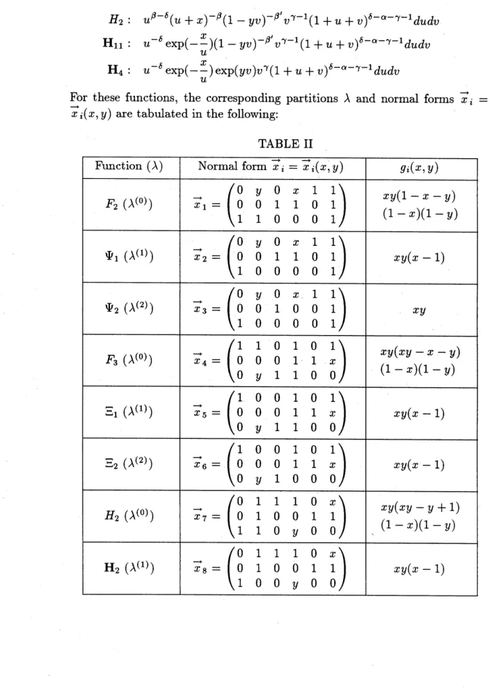
For these functions, the corresponding partitions $\lambda$ and normal $\mathrm{f}\mathrm{o}\mathrm{r}\mathrm{m}\mathrm{S}arrow x_{i}=$
$arrow x_{i}(x, y)$ are tabulated in the following:
For the normal $\mathrm{f}\mathrm{o}\mathrm{r}\mathrm{m}\mathrm{S}arrow x_{i}=arrow x_{i}(X, y)$, the
$\mathrm{v}\mathrm{a}\mathrm{r}\mathrm{i}\mathrm{a}\mathrm{b}.\cdot 1$es $(x, y)\in \mathbb{C}^{2}$ are subject to
the condition $g_{i}(X, y)\neq 0$.
Proposition 4.1. Let $\lambda^{(\nu)}$
and the normal forms $x_{i}arrow=arrow x_{i}(X, y)$ begiven in
Table III. The $CHG$ functions on $GL(3)\backslash Z^{\nu}/H_{\lambda^{(\nu)}}$ with the normalized
pa-ramet$\mathrm{e}rs\beta_{\nu}(0\leq\nu\leq 3)$arerelated with the classi$c\mathrm{a}l$hypergeometric functions
oftwo variables, for instence, $as$
$\Phi_{\lambda^{(0)}}(_{X_{1;}}arrow\beta 0)=\int_{\Delta_{1}}.v^{\alpha_{0}}(v+y)^{\alpha}1\alpha_{2}uu(+x)^{\alpha_{3}}(1+u+v)\alpha_{5}dudv$
$=C1F2(\alpha 4+1, -\alpha_{3}, -\alpha_{1}, -\alpha 2-\alpha 3, -\alpha 0-\alpha 1;x, y)$
$\Phi_{\lambda^{(1)}}(^{arrow}x_{2}; \beta_{1})=\int_{\triangle_{2}}v\exp u^{\alpha_{2}}(u+x)^{\alpha}3(1+u+v)\alpha 0\alpha \mathrm{s}dudv$
$=C_{2}\Psi 1(\alpha_{4}+1, -\alpha_{3}, -\alpha 3^{-\alpha}2, -\alpha 0;x, y)$
$\Phi_{\lambda^{(2)}}(x_{3}arrow; \beta 2)=\int_{\Delta_{3}}v^{\alpha_{0}}\exp(-\frac{y}{v})u\alpha_{2}\exp(-\frac{x}{u})(1+u+v)^{\alpha_{5}}dudv$
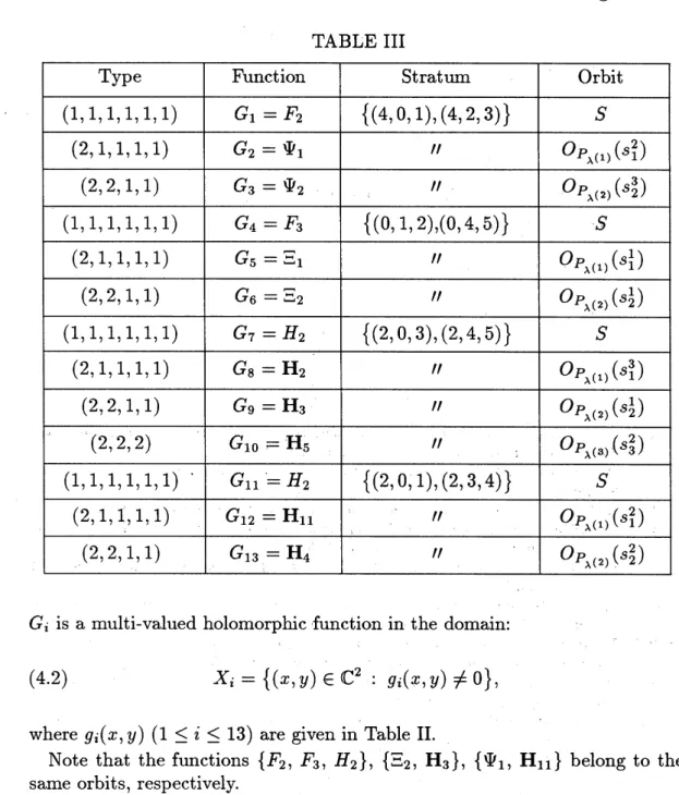
The properties of those functions can be described in the following Table. TABLE III
$G_{i}$ is a multi-valued holomorphic function in the domain:
(4.2) $X_{i}=\{(x, y)\in \mathbb{C}2 : g_{i}(x, y)\neq 0\}$,
where $g_{i}(X, y)(1\leq i\leq 13)$ are given in Table II.
Note that the functions $\{F_{2}, F_{3}, H_{2}\},$
{
$-$ ,H3},
$\{\Psi_{1}, \mathrm{H}_{11}\}$ belong to thesame orbits, respectively.
\S 5
$\mathrm{n}_{\mathrm{a}\mathrm{n}\mathrm{S}}\mathrm{f}\mathrm{o}\mathrm{r}\mathrm{m}\mathrm{a}\mathrm{t}\mathrm{i}\mathrm{o}\mathrm{n}$ formulae.We systematically deduce some transfomation fomulae for the systems of
$F_{3}(\alpha, \alpha’, \beta, \beta’, \gamma;x, y)$
$=x^{-\rho\beta’}y^{-}F2( \beta+\beta’-\gamma+1, \beta, \beta’, \beta-\alpha+1, \beta’-\alpha’+1;\frac{1}{x}, \frac{1}{y})$.
$H_{2}(\alpha, \beta, \beta’,\gamma, \delta;X, y)$
$=y^{-\beta’}F2( \alpha+\beta’, \beta, \beta’, \delta, \beta’-\gamma+1;x, -\frac{1}{y})$,
$F_{3}(\alpha, \alpha’, \beta, \beta’, \gamma;X, y)$
$=x^{-\alpha_{H_{2}}}( \alpha-\gamma+1, \alpha, \alpha’, \beta J, \alpha-\beta+1;\frac{1}{x}, -y)$,
$\mathrm{H}_{11}(\alpha, \beta’, \gamma, \delta;x, y)$
$=y^{-\rho_{\Psi_{1}}’}( \alpha+\beta’, \beta’, \beta’-\gamma+1, \delta;-\frac{1}{y}, x)$,
H3
$(\alpha, \beta, \delta;x, y)$$=x^{-\beta}---_{2}( \beta, \beta-\delta+1, -\alpha+\beta+1;\frac{1}{x}, -y)$
.
REFERENCES
[A-K] P. Appell&J. Kamp\’edeFeriet, Fonctions Hyperge’ometfiques et
Hyperspheriques-Polynomes d’Hermite I, Gauther-Villars. Paris (1926).
[D-L] B. Dwork &F. Loeser, Hypergeometric $se\dot{\sim}es$, Japan. J. Math. 19, No.l (1993),
81-129.
[Erd 1] A. Erd\’elyi, Higher $\pi_{anS}cendenta\iota$ Functions, vol. 1, $\mathrm{M}\mathrm{c}\mathrm{G}\mathrm{r}\mathrm{a}\mathrm{w}$-Hill, 1953.
[Erd 2] A. Erd\’elyi, Transformations ofhypergeometricfunctionoftwovariables, Proc. Roy.
Soc. Edinburgh Sect. A 62 (1948), 378-385.
[G] I.M. Gel’fand, Generaltheory ofhypergeometricfunctions, Soviet. Math. Dokl. 33
(1986), 573-577.
[Ki] M. Kita, On hypergeometricfunctions in several variables 1. New integral
repre-sentations ofEuler type,Japan. J. Math. 18, No.1 (1992), 25-74.
[K-H-T] H. Kimura&Y. Haraoka&K. Takano, The generalized confluent hypergeometric functions, Proc. Japan Acad. 68, Ser. A (1992), 290-295.
[K-K] H. Kimura&T. Koitabashi, Normalizer of maximal abelian group of$GL(n)$ and
confluent hypergeometric function, preprint (1994).
[O-K] K. Okamoto &H. Kimura, On particular solutions of Garnier systems and the
hypergeometricfunctions ofseveralvariabfes, Quarterly J. Math. 37 (1986), 61-80.
[Y] M. Yoshida, Eulerintegraltransformations ofhypergeometricfunctions oftwo vari-ables, Hiroshima Math. J. 10 (1980), 329-335.
GRADUATE SCHOOL OF MATHEMATICAL SCIENCES, THE UNIVERSITY OF TOKYO, 3-8-1