The application of PVM to the computation of vortex sheet motion(Domain Decomposition Methods and Related Topics)

The

application

of PVM

to the

computation

of

vortex

sheet

motion

Hisashi

OKAMOTO

and Takashi

SAKAJO

Research Institute for Mathematical Sciences,

Kyoto

University,

Kyoto,

606-01,

Japan

1

Vortex

sheet and

its governing

equation

We consider a motion ofincompressible, inviscid fluid. Attention is restricted to avortex

sheet motion. A vortex sheet is a surface, along which the velocity changes

discontinu-ously. Thevorticity concentrates onthe surface, outside whichthe flowis irrotational. We

assume a further simplification that the flow is two-dimensional. Mathematically,

two-dimensional vortex sheet is representedbya

curve.

Whenweidentify the two-dimensional

space with complex plane, avortex sheet intwo-dimensional space is expressed bya

com-plex valued function $z(\Gamma,t)$, where $\Gamma\in \mathrm{R}$ is a Lagrangian parameter along the curve,

which represents the circulation of the flow. $t$ represents time.

We consider thedynamicsofa two-dimensional vortexsheet with a $\mathrm{p}$

.eriodic

boundary condition;

$z(\Gamma+1, t)=z(\mathrm{r}, t)+1$

.

The equationwhich describesthe motionofvortexsheet isknown

as

the Birkhoff-Rott

equation([16]):

$\frac{\partial z^{*}(\Gamma,t)}{\partial t}=\frac{1}{2\pi i}\mathrm{p}.\mathrm{v}$

.

$\int\frac{d\Gamma’}{z(\Gamma,t)-z(\Gamma’,t)}$

The integral on the right hand side is Cauchy’s principal value. $i$ is the imaginary un\‘it.

$*\mathrm{d}\mathrm{e}\mathrm{n}\mathrm{o}\mathrm{t}\mathrm{e}\mathrm{S}$ complex conjugate. Taking the

periodic boundary condition into account, we rewrite the equation and obtain$([8])$:

$\frac{\partial z^{*}(\Gamma,l)}{\partial t}$

$=$ $\frac{1}{2i}\mathrm{p}.\mathrm{v}$

.

$\int_{0}^{1}\cot\pi(Z(\Gamma, t)-z(\Gamma’, t))d\mathrm{r}’$.

This is the equation which we are going to study numerically.

A flat vortex sheet of constant strength, $z(\Gamma, t)\equiv\Gamma$, is

an

equilibrium solution of the

equation (1). This equilibrium is known to be unstable: even a small perturbation can grows very rapidly and thevortex sheet shows extreme complexity for large$t([8,9,17])$

.

The following properties are known:

$\bullet$ Linearized stability analysis shows that perturbations of short

wave

length grow

exponentially. The shorter the wavelength is,thefaster theperturbationgrows$([16])$.

(Kelvin-Helmholtz instability.)

$\bullet$ If the initialperturbationisananalyticfunction of$\Gamma$, then thesheetremainsanalytic

for a positive time interval ([2, 20]).

$\bullet$ The vortex sheet loses analyticity in finite time$([14])$

.

$\bullet$ The initial value problem for (1) is ill-posed in the sense of Hadamard$([3])$

.

$\bullet$ A vortex sheet evolves into a complex form having spirals (see,

for.

instance, [8, 9, 17]).

Because of the ill-posedness of the equation, it is difficult to apply naive numerical

methods to the computation of a vortex sheet. We apply Chorin’s vortex blob method,

which we

are

going to explain in the next section.

2

Numerical method

Instead of the original equation, we consider the following smoothed equation. (This

equation is given by Krasny$([8])$

.

).

$\frac{\partial z^{*}(\Gamma,t)}{\partial t}=\int_{0}^{1}K_{\delta}(z(\mathrm{r}, t)-Z(\Gamma’, t))d\Gamma’$, (2)

where

$K_{\delta}(X+ \dot{i}y)=-\frac{1}{2}\frac{\sinh(2\pi y)+i\sin(2\pi x)}{\cosh(2\pi y)-\cos(2\pi x)+\delta^{2}}$.

This equation is well-posedfor any time interval if$\delta>0$. $\delta$ is an artificial parameter

that makesthe equation well-posed. When$\delta=0$, the equationreducestothe original equation.

The convergence of the solution of the smoothed equation to that of the Birkhoff-Rott

equation is proven as far asthe solution of (1) is smooth. However, after the appearance

2.1

Discretization

In order to compute (2), we approximate the

vorte.x

sheet by $N$ points.

$\Gamma_{i}=\frac{i}{N}$, $z(\Gamma_{i}, t)=z_{i}(t)$, $i=0,$ _$\cdots,$$N-1$

.

Then, we discretize the integral by trapezoidal rule and obtain the following system of

ordinary differential equations:

$\frac{\partial z_{n}^{*}(t)}{\partial t}=\frac{1}{N}\sum_{m=0}^{N}K_{\delta}(_{Z_{n}}(-1t)-zm(t))$, $i=0,$

$\cdots,$$N-1$

.

(3)

In order to integrate the system of O.D.E, we

use

the fourth-order Runge-Kutta method.

The parameters we can change are as follows:

$\bullet$ $N\cdots$ the number of vortices

$\bullet$ $\triangle t\cdots$ time step size for Runge-Kutta method $\bullet$ $\delta\cdots$ smoothing parameter of vortex blob method

This

is a rough description ofthevortex method. For more details, see, e.g., Puckett [15].

Numerical computationofthe right hand side of(3) requires $O(N)$ multiplications for

each vortexpoint. Since thereare $N$vortices, $O(N^{2})$ operationsare necessary to compute

the velocityfields at all the positionsofparticles. Inorder toobtain an accurate numerical

solution, we need a large number of vortices to discretize the vortex sheet. Thus the

computation becomes too slow when $N$ is large. This is the most serious disadvantage

of the vortex method. There are

some

algorithms which evaluate the velocity field in

$O(N\log N)$ operations within

some errors

_{$([4,6,7,18])$}

.

Although _they

are

_promising,

theyhave some defects, too$([7,18])$. In the present paper, we _{would like to study another}

method, Parallel Virtual Machine software, to evaluate the velocity field at the vortex points. In the following section, we will explain how to implement this tool for numerical computations and the efficiency will be examined.

3

Parallel

Virtual Machine

The ParallelVirtual Machine (shortly PVM) is a software framework for heterogeneous

parallel computing in networked environments ([5]). PVM supports complete message

passing model and it emulates a distributed memory model in heterogeneous network.

Our virtual parallel machine consists of four computers. They have the following

CPU’s, memory, and operating systems, respectively

$\bullet$ $\mathrm{B}\cdots$ Pentium

$120\mathrm{M}\mathrm{H}\mathrm{Z},$ $64\mathrm{M}\mathrm{B}$, FREEBSD

$\bullet$ $\mathrm{C}\cdots$ Pentium $100\mathrm{M}\mathrm{H}_{\mathrm{Z},6}4\mathrm{M}\mathrm{B}$, FREEBSD

$\bullet$ $\mathrm{D}\cdots$ Pentium$60\mathrm{M}\mathrm{H}\mathrm{Z},$ $24\mathrm{M}\mathrm{B}$, FREEBSD

These computers

are

connected through 10Base-T Ethernet.

We

use

the following master-slave type algorithm to implement the $\mathrm{c}$

.omputation

of

velocity field:

1. Divide $N$ points by $k$ group ( $k$ is the number of computers).

$n_{j}$ is the number

of vortices, the velocities of which are computed in the j-th computer, whence

$\Sigma_{j=1j}^{k}n=N$

.

2. Send the position of$n_{j}$ vortices to each slave computers

3. Each slave computer evaluates the velocities at the positions of $n_{j}$ points

4.

_S.

end back the results to the master computer

5. loop to 2

$n_{j}$ is determined by CPU speed to make the evaluation time of each computers as even

as possible.

3.1

Test

problem

:

Two

Vortex Sheets

Using PVM and vortex blob method for a vortex sheet, we compute the motion of two

vortex sheets. We consider two, nearly parallel, vortex sheets. We denotes upper vortex sheet and lower vortex sheet by $z(\Gamma, t)$ and $w(\Gamma, t)$, respectively. Then the equation of

motion of two vortex sheets is written as follows:

$\frac{\partial Z^{*}(\Gamma,t)}{\partial t}$ _{$=$ $\frac{\sigma_{1}}{2_{\dot{i}}}\mathrm{p}.\mathrm{v}.\int_{0}^{1}\cot\pi(Z(\Gamma, t)-z(\mathrm{r}’, t))d\mathrm{r}$}’

$+$ $\frac{\sigma_{2}}{2i}\int_{0}^{1}\cot\pi(Z(\Gamma, t)-w(\Gamma’, t))d\mathrm{r}’$,

$\frac{\partial w^{*}(\Gamma,t)}{\partial t}$

$=$ $\frac{\sigma_{2}}{2i}\mathrm{p}.\mathrm{v}.\int_{0}^{1}\cot\pi(w(\Gamma, t)-w(\Gamma’, t))d\Gamma’$

$+$ $\frac{\sigma_{1}}{2i}\int_{0}^{1}\cot\pi(w(\mathrm{r}, t)-Z(\Gamma’, t))d\Gamma’$,

where $\sigma_{1}$ is the vorticity densityof upper vortex sheet and

The initial value of$z$ and $w$ is taken

as

follows:

$z(\Gamma, \mathrm{O})$ $=$ $\Gamma+\epsilon\sin 2\pi \mathrm{r}-i\epsilon\sin 2\pi\Gamma+i\frac{H}{2}$ ,

$w(\Gamma, 0)$ $=$ $\Gamma+\epsilon\sin 2\pi\Gamma-i\epsilon\sin 2\pi(\Gamma+\alpha)-\dot{i}\frac{H}{2}$

$(0\leq\alpha<1, H\neq 0,0\leq\Gamma<1)$,

where $H$ is average distance between two vortex sheets and a is the phase difference of

two vortexsheets.

The numerical parameters ofthe computations are

$\bullet$ $N\cdots$ the number of vortices

$\bullet$ $\Delta t\cdots$ time step size for Runge-Kutta method $\bullet$ $\delta\cdots$ smoothing parameter of vortex blob method $\bullet$ $\epsilon\cdot\cdot$

. $\cdot$ the amplitude of the disturbance

$\bullet$ $H\cdots$ the average distance between two vortex sheets $\bullet$ $\alpha\cdots$ initial phase difference oftwo vortex sheets

$\bullet$

$\sigma_{1},\sigma_{2}\cdots$ the vorticity oftwo vortex sheets.

3.2

Reduction of

execution

time

We show the execution time when we

use

PVM. The execution time (in second) is

mea-sured by

one

time step of Runge-Kuttamethod. (Thetime to evaluatevelocityfield four

times. ) Among four computers, machine $\mathrm{B}$ is the fastest of the four computers. The

ratio of CPU speeds is approximately equal to $\mathrm{A}:\mathrm{B}:\mathrm{c}:\mathrm{D}=9:10:8:5$

.

We divide $N$ vortex

points according as this ratio. The following are the list of of performances. 3.2.1 The result for $N=2048$

1. Single processor $k=1$

$\bullet$ $\mathrm{A}\cdots$ 40.68 seconds $\bullet$ $\mathrm{B}\cdots$ 33.79 seconds $\bullet$ $\mathrm{C}\cdots$ 41.19 seconds $\bullet$ $\mathrm{D}\cdots$ 67.22 seconds

$\bullet$ $\mathrm{A}+\mathrm{B}\cdots$ 20.87 seconds $(\cross 1.62)$

3. Three processors $k=3$

$\bullet$ $\mathrm{A}+\mathrm{B}+\mathrm{C}\cdots$ 14.81 seconds $(\cross 2.28)$

4. Four processors $k=4$

$\bullet$ $\mathrm{A}+\mathrm{B}+\mathrm{C}+\mathrm{D}\cdots$ 13.26 seconds $(\cross 2.54)$

Here and hereafter, $\cross 1.77$, for instance, implies that the computation is 1.77 times faster than the computation of single $\mathrm{B}$ processor.

3.2.2 The result for $N=4096$

1. Single processor

$\bullet$ $\mathrm{A}\cdots$ 153.09 seconds $\bullet$ $\mathrm{B}\cdot\cdot$ ‘ 134.98 seconds $\bullet$ $\mathrm{C}\cdots$ 263.29 seconds $\bullet$ $\mathrm{D}\cdots$ 159.49 seconds

2. Two processors

$\bullet$ $\mathrm{A}+\mathrm{B}\cdots$ 75.90 seconds $(\cross 1.77)$

3. Three processors

$\bullet$ $\mathrm{A}+\mathrm{B}+\mathrm{C}\cdots$ 55.29 seconds $(\cross 2.44)$

4. Four processors

$\bullet$ $\mathrm{A}+\mathrm{B}+\mathrm{c}+\mathrm{D}\cdots$49.19 seconds $(\cross 2.74)$

$3.2.3$ The result for _$N=8192$

1. Single processor

$\bullet$ $\mathrm{A}\cdots$ 635.06 seconds $\bullet$ $\mathrm{B}\cdots$ 521.05 seconds $\bullet$ $\mathrm{C}\cdots$ 640.54 seconds $\bullet$ $\mathrm{D}\cdots$ 1050.41 seconds

$\bullet$ $\mathrm{A}+\mathrm{B}\cdots$

308.12

seconds $(\cross 1.69)$

3. Three processors

$\bullet$ $\mathrm{A}+\mathrm{B}+\mathrm{C}\cdots$ 219.82 seconds $(\cross 2.37)$

4. Four processors

$\bullet$ $\mathrm{A}+\mathrm{B}+\mathrm{C}+\mathrm{D}\cdots$ 188.56 seconds $(\cross 2.76)$

The above results show that the usefulness of PVM at least when a small number of

computers are combined.

3.3

Numerical

results

We choose $N=4096$

.

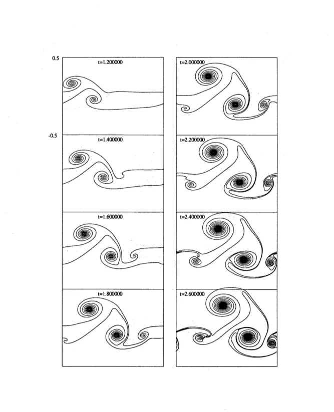
Figure 1 is the long time evolution of two vortex sheets. Initial

averagedistance $H$ is 0.2, initial phasedifference a is O,and $(\sigma_{1}, \sigma_{2})=(1, -1)$

.

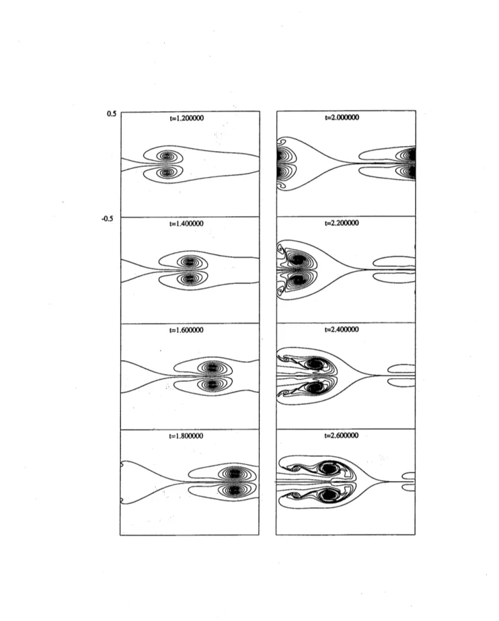
Figure 2 is

thelongtime evolution of twovortexsheets. Initialaveragedistance$H$is 0.2, initialphase

difference $\alpha$is 0.$5,\mathrm{a}\mathrm{n}\mathrm{d}(\sigma_{1}, \sigma_{2})=(1, -1)$

.

Bothfigures show complicated spiral structures.

Since the vorticity is not of distinguished sign $(\sigma_{1}, \sigma_{2})=(1, -1)$, such complexities

seem

to comply with what are predicted in [13].

4

Summary

and

acknowledgment

When the number of vortices exceeds a few thousands, the efficiency of PVM is

satis-factory. PVM is a useful tool for particle simulations. However, if PVM environment

consists of a lot of node computers, the rapid increase of data transfer may well make

it impossible for

us

to execute fast computation. To make more efficient computation,

we must choose algorithms with more effective data transfer. There is a possibility to

combine the fast algorithms $[4, 6]$ and PVM effectively.

Professor O. Pironneau advised us to try computations with adaptive increase of the

numberof vortices. This attempt isin progress andwill be reportedelsewhere. We thank

Figure 1: Long time evolution oftwo vortex sheets. The initial parameters are $H=0.2$, $\alpha=0.0,\mathrm{a}\mathrm{n}\mathrm{d}(\sigma_{1}, \sigma_{2})=(1, -1)$.

Figure 2: Long time evolution of two vortex sheets. The initial parameters are $H=0.2$,

References

[1] C. B\"ogers, On the numerical solution of the regularized Birkhoff equation, Math.

Comp. vol. 53 (1989), pp. 141-156.

[2] R.E. Caflisch and O.F. Orellana, Longtime existence for a slightly perturbed vortex

sheet, Comm. Pure Appl. Math., vol. 39 (1986), pp. 807-838.

[3] R.E. Caflisch andO.F.Orellana, Singular solutionsand ill-posednessfor the evolution

ofvortex sheets, SIAM J. Math. Anal., vol. 20 (1989), pp. 293-307.

[4] C. I. Draghicescu, An efficientimplementationofparticle methodsfor the

incompress-ible Euler equations, SIAM J. Numer. Anal., vol. 31, $\mathrm{N}\mathrm{o}.4(1994)$, pp. 1090-1108.

[5] A. Geist et at., PVM:Parallel Virtual Machine, MIT Press, 1994.

[6] L. Greengard and V. Rokhlin, A fast algorithm for particle simulations, J. Comput. Phys. vol. 73(1987), pp. 325-348.

[7] J.T. Hamilton and G. Majda, On the Rokhlin-Greengard method with vortex blobs

for problems posed in all space or periodic in one direction, J. Comput. Phys. vol. 121(1995), pp. 29-50.

[8] R. Krasny, Desingularization of periodic vortex sheet roll-up , J. Comp. Phys., vol.

65 (1986), pp. 292-313.

[9] R. Krasny, Computation ofvortex sheet roll-up, SpringerLecture Notes in Math., $\#$ 1360 (1988), pp. 9-22.

[10] R. Krasny,VortexDynamics and Vortex Methods, eds., C.R. Andersonand C.

Green-gard, Lectures in Applied Mathematics Amer. Math. Soc. (1991), vol. 28, pp. 385-402.

[11] C. Lin and L. Sirovich, Nonlinear vortex trail dynamics , Phys. Fluids vol. 31 (1988),

pp. 991-998.

[12] J.G. Liu and Z. Xin, Convergence of vortex methods for weak solutions to the 2-D

Euler equations with vortex sheet data, Comm. Pure Appl. Math., vol. 48 (1995),

pp. 611-628.

[13] A.J. Majda, Remarks on weak solutions for vortex sheets with a distinguished sign,

Indiana Univ. Math. J., vol. 42 (1993), pp. 921-939.

[14] D.W. Moore, Thespontaneousappearance ofasingularityinthe shapeofanevolving

[15] E.G. Puckett, Vortex methods: An introduction and survey of selected research

topics, in “ _{Incompressible Computational Fluid Dynamics Trends and Advances,}

eds. M.D. Gunzburger$\dot{\mathrm{a}}$

ndR.A. Nicolaides, Cambridge Univ. Press, (1993), pp. 335-407.

[16] P.G. Saffman, Vortex Dynamics, Cambridge Univ. Press, (1992).

[1.7]

T. Sakajo and H. Okamoto, Numerical computation of vortex sheet roll-up in the

background shear flow, Fluid Dynamics Research vo117 (1995), pp. 101-119.

[18] T. Sakajo and H. Okamoto, An applicationof Draghicescu’s fast summation method

to vortex sheet motion, to appear in RIMS Kokyuroku, ed. Y. Kaneda.

[19] T. Sakajo, Interactions oftwovortex sheets, acceptedfor publication byAdv. Math.

Sci. Appl.

[20] C. Sulem et al., Finite time analyticity for the two and three dimensional