JAIST Repository: Laminar Structure of Ptolemaic Graphs with Applications

(1)

JAIST Repository

https://dspace.jaist.ac.jp/

Title Laminar Structure of Ptolemaic Graphs with Applications

Author(s) Uehara, Ryuhei; Uno, Yushi

Citation Discrete Applied Mathematics, 157(7): 1533-1543 Issue Date 2008-10-23

Type Journal Article

Text version author

URL http://hdl.handle.net/10119/9180

Rights

NOTICE: This is the author’s version of a work accepted for publication by Elsevier. Changes resulting from the publishing process, including peer review, editing, corrections, structural formatting and other quality control mechanisms, may not be reflected in this document. Changes may have been made to this work since it was submitted for publication. A definitive version was subsequently published in Ryuhei Uehara and Yushi Uno, Discrete Applied Mathematics, 157(7), 2008, 1533-1543,

http://dx.doi.org/10.1016/j.dam.2008.09.006 Description

(2)

Laminar Structure of Ptolemaic Graphs with

Applications ?

Ryuhei Uehara

a

and Yushi Uno

b

a _{School of Information Science, Japan Advanced Institute of Science and} Technology (JAIST), Ishikawa, Japan.

b _{Department of Mathematics and Information Sciences, Gradate School of} Science, Osaka Prefecture University, Osaka, Japan.

Abstract

Ptolemaic graphs are those satisfying the Ptolemaic inequality for any four ver-tices. The graph class coincides with the intersection of chordal graphs and distance hereditary graphs. It can also be seen as a natural generalization of block graphs (and hence trees). In this paper, we first state a laminar structure of cliques, which leads to its canonical tree representation. This result is a translation of γ-acyclicity which appears in the context of relational database schemes. The tree representation gives a simple intersection model of ptolemaic graphs, and it is constructed in lin-ear time from a perfect elimination ordering obtained by the lexicographic breadth first search. Hence the recognition and the graph isomorphism for ptolemaic graphs can be solved in linear time. Using the tree representation, we also give an efficient algorithm for the Hamiltonian cycle problem.

Key words: Algorithmic graph theory, data structures, γ-acyclicity, Hamiltonian

cycle, intersection model, ptolemaic graphs.

1 Introduction

From an algorithmic point of view, a variety of graph classes have been pro-posed and studied so far [4,17]. Among them, the class of chordal graphs is

? Preliminary version was presented at the 16th Annual International Symposium

on Algorithms and Computation (ISAAC 2005)[32].

Email addresses: [email protected] (Ryuhei Uehara),

(3)

classic and widely investigated. One of the reasons is that the class has a nat-ural intersection model and hence has a concise tree representation; that is, a graph is chordal if and only if it is the intersection graph of subtrees of a tree. The tree representation can be constructed in linear time, and the tree is called a clique tree since each node of the tree corresponds to a maximal clique of the chordal graph (see [29]). Another reason is that the class is char-acterized by a vertex ordering, which is called a perfect elimination ordering. The ordering can also be computed in linear time, and a typical way to find it is called the lexicographic breadth first search (LBFS) introduced by Rose, Tarjan, and Lueker [28]. The LBFS is also intensively investigated as a tool for recognizing several graph classes (see a comprehensive survey by Corneil [9]). Using those characterizations, many efficient algorithms have been established for chordal graphs; to list a few of them, the maximum weighted clique prob-lem, the maximum weighted independent set probprob-lem, the minimum coloring problem [16], the minimum maximal independent set problem [15], and so on. There are also parallel algorithms to solve some of these problems efficiently [24].

In algorithmic graph theory, distance in graphs is one of the most important topics. The class of distance hereditary graphs was characterized by Howorka to deal with the distance property called isometric [19]. Some characteriza-tions of distance hereditary graphs are also given by Bandelt and Mulder [1], D’Atri and Moscarini [12], and Hammer and Maﬀray [18]. Especially, Bandelt and Mulder showed that any distance hereditary graph can be obtained from

K2 by a sequence of extensions called “adding a pendant vertex” and

“split-ting a vertex.” Using these characterizations, many efficient algorithms have been found for distance hereditary graphs [3,6–8,22,23,27]. Among them, a few linear time algorithms are known for the recognition of a distance hereditary graph, however, they are too complicated and far from practical; Hammer and Maffray’s algorithm [18] fails in some cases, and Damiand, Habib, and Paul’s algorithm [11] requires to build a cotree in linear time (see [11, Chapter 4] for further details), where the cotree can be constructed in linear time by using a classic algorithm due to Corneil, Perl, and Stewart [10], or a recent algorithm based on multisweep LBFS approach by Bretscher, Corneil, Habib, and Paul [5]. Recently, Nakano, Uehara, and Uno also give another linear time algorithm for the recognition of distance hereditary graphs, which maintains two neighbor sets by two prefix trees [23]. However, their algorithm requires delicate implementation to achieve linear time.

In this paper, we focus on the class of ptolemaic graphs. Ptolemaic graphs are graphs that satisfy the Ptolemaic inequality d(x, y)d(z, w)≤ d(x, z)d(y, w) +

d(x, w)d(y, z) for any four vertices x, y, z, w. (The inequality is also known as

“Ptolemy” inequality which seems to be more popular. However we use “Ptole-maic,” which is stated by Howorka [20].) Howorka showed that the class of ptolemaic graphs coincides with the intersection of the class of chordal graphs

(4)

and the class of distance hereditary graphs [20]. Hence the results for chordal graphs and distance hereditary graphs can be applied to ptolemaic graphs. On the other hand, the class of ptolemaic graphs is a natural generalization of block graphs, and hence trees (see [33] for the relationships between related graph classes). However, there are relatively few known results speciﬁed to ptolemaic graphs.

We first state a tree representation of ptolemaic graphs which is based on the laminar structure of cliques of a ptolemaic graph. We here note that this result itself is not necessarily new. In [13], D’Atri and Moscarini showed that chordal graphs and its subclasses are strongly related to acyclicity concepts for hypergraphs which appeared in relational database theory. Especially, a ptolemaic graph corresponds to a γ-acyclic hypergraph, which is introduced by Fagin in [14]. The γ-acyclicity of hypergraph directly corresponds to the tree structure in our paper. The tree representation also gives a natural in-tersection model for ptolemaic graphs, which is defined over directed trees. We show a linear time algorithm that constructs the tree representation for a ptolemaic graph. The construction algorithm can also be modified to a recog-nition algorithm which runs in linear time. It is worth remarking that the algorithm is quite simple, especially, much simpler than the combination of two recognition algorithms for chordal graphs and distance hereditary graphs. In the tree construction and the recognition, the ordering of the vertices pro-duced by the LBFS plays an important role. Therefore, our result adds the class of ptolemaic graphs to the list of graph classes that can be recognized efficiently by the LBFS. Moreover, the tree representation is canonical up to isomorphism. Hence, using the tree representation, we can solve the graph iso-morphism problem for ptolemaic graphs in O(|V | ) time if a ptolemaic graph is given in the tree representation. We note that a clique tree of a chordal graph is not canonical and the graph isomorphism problem for chordal graphs is graph isomorphism complete.

The tree representation enables us to use the dynamic programming tech-nique for some problems on ptolemaic graphs G = (V, E). It is sure that the Hamiltonian cycle problem is one of most well known NP-hard problem, and it is still NP-hard even for a chordal graph, and that an O(|V | + |E| ) time algorithm is known for distance hereditary graphs [21,22]. In this paper, we show that the Hamiltonian cycle problem can be solved in O(|V | ) time by using the technique if a ptolemaic graph is given in the tree representation. As we mentioned, the tree structure of a ptolemaic graph is known as γ-acyclicity for corresponding hypergraph in relational database theory, and it produces loop-free Bachman diagram (see [2,14] for more details). In a γ-acyclic hypergraph, hyperedges correspond to maximal cliques in ptolemaic graph. In [14], Fagin mentioned that the hypergraph can be recognized in polynomial time. Hence, we can say that our algorithm can also be used as a

(5)

more eﬃcient substitution to recognize the hypergraphs in relational database theory.

2 Preliminaries

The neighborhood of a vertex v in a graph G = (V, E) is the set NG(v) =

{u ∈ V | {u, v} ∈ E}, and the degree of a vertex v is |NG(v)| and is denoted

by deg_G(v). For a subset U of V, we denote by NG(U ) the set {v ∈ V |

v ∈ N(u) for some u ∈ U}. If no confusion can arise we will omit the index G. Given a graph G = (V, E) and a subset U of V , the induced subgraph

by U , denoted by G[U ], is the graph (U, E0), where E0 = {{u, v} | u, v ∈

U and {u, v} ∈ E}. Given a graph G = (V, E), its complement, denoted by

¯

G = (V, ¯E), is deﬁned by ¯E = {{u, v} | {u, v} 6∈ E}. A vertex set I is an independent set if G[I] contains no edges, and then the graph ¯G[I] is said to

be a clique.

Given a graph G = (V, E), a sequence of the distinct vertices v1, v2, . . . , vl is

a path, denoted by (v1, v2, . . . , vl), if {vj, vj+1} ∈ E for each 1 ≤ j < l. The

length of a path is the number of edges in the path. For two vertices u and v,

the distance of the vertices, denoted by d(u, v), is the minimum length of the paths joining u and v. A cycle is a path beginning and ending at the same vertex. A cycle is said to be Hamiltonian if it visits every vertex in a graph exactly once.

An edge which joins two vertices of a cycle but is not itself an edge of the cycle is a chord of that cycle. A graph is chordal if each cycle of length at least 4 has a chord. Given a graph G = (V, E), a vertex v ∈ V is simplicial in G if G[N (v)] is a clique in G. An ordering v1, . . . , vn of the vertices of

V is a perfect elimination ordering (PEO) of G if the vertex vi is simplicial

in G[{vi, vi+1, . . . , vn}] for all i = 1, . . . , n. Once a vertex ordering is ﬁxed, we

denote N (vj)∩{vi+1, . . . , vn} by N>i(vj). We also use the notations “min” and

“max” to denote the first and the last vertices in an ordered set of vertices, respectively. It is known that a graph is chordal if and only if it has a PEO (see [4, Section 1.2] for further details). A typical way of finding a perfect elimination ordering of a chordal graph in linear time is the lexicographic breadth first search (LBFS), which is introduced by Rose, Tarjan, and Lueker [28], and a comprehensive survey is presented by Corneil [9].

It is also known that a graph G = (V, E) is chordal if and only if it is the intersection graph of subtrees of a tree T (see [4, Section 1.2] for further details). Let Tv denote the subtree of T corresponding to the vertex v in G.

Then we can assume that each node c in T corresponds to a maximal clique

(6)

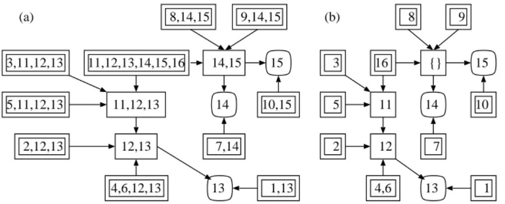
16 12 4,6 9 11 {} 14 15 7 8 10 5 (b) 3 2 13 1 11,12,13,14,15,16 12,13 4,6,12,13 9,14,15 11,12,13 14,15 14 15 7,14 8,14,15 10,15 5,11,12,13 (a) 3,11,12,13 2,12,13 13 1,13

Fig. 1. (a) Laminar tree; (b) its labels

a tree T is called a clique tree of G. From a perfect elimination ordering of a chordal graph G, we can construct a clique tree of G in linear time [29]. We sometimes identify a node c of a clique tree T with a maximal clique (or a vertex set) C of G.

Given a graph G = (V, E) and a subset U of V , an induced connected subgraph

G[U ] is isometric if the distances in G[U ] are the same as in G. A graph G is distance hereditary if G is connected and every induced path in G is isometric.

A connected graph G is ptolemaic if for any four vertices u, v, w, x of G,

d(u, v)d(w, x)≤ d(u, w)d(v, x)+d(u, x)d(v, w). We will use the following

char-acterization of ptolemaic graphs due to Howorka [20]:

Theorem 1 The following conditions are equivalent: (1) G is ptolemaic; (2)

G is distance hereditary and chordal; (3) for all distinct nondisjoint maximal cliques P and Q of G, P ∩ Q separates P \ Q and Q \ P .

Let V be a set of n vertices. Two sets X and Y are said to be overlapping if

X∩ Y 6= ∅, X \ Y 6= ∅, and Y \ X 6= ∅. A family F ⊆ 2V \ {{∅}} is said to

be laminar if F contains no overlapping sets; that is, any pair of two distinct sets X and Y in F satisﬁes either X ∩ Y = ∅, X ⊂ Y , or Y ⊂ X. Given a laminar familyF, we deﬁne laminar digraph −→T (F) = (F, −→E_F) as follows;−→E_F

contains an arc (Y, X) if and only if X ⊂ Y and there are no other subset Z ofF such that X ⊂ Z ⊂ Y , for any sets X and Y . In this case, Y is said to be

parent of X, and X is said to be child of Y . We denote the underlying graph

of −→T (F) by T (F) = (F, E_F). The following lemma for the laminar digraph is known (see, e.g., [26, Chapter 2.2]);

Lemma 2 If a family F ⊆ 2V \ {{∅}} is laminar, (1) T (F) is a forest, and

(2) |F| ≤ 2 |V | − 1.

Hence, hereafter, we call T (F) (−→T (F)) a (directed) laminar forest. On a

di-rected laminar forest −→T (F), we abuse some notations for trees as follows; we

(7)

leaf can have two or more parents if it has indegree two or more. To have a compact representation, we deﬁne a label of each node S0 in F of −→T (F),

denoted by `(S0), as follows: If S0 is a leaf, `(S0) = S0. If S0 is not a leaf and

has children S1, S2, . . . , Sh, `(S0) = S0\(S1∪S2∪· · ·∪Sh). That is, each vertex

v in V appears in `(S) where S is the minimal set containing v. Since F is

laminar, each vertex in V appears exactly once in `(S) for some S ⊆ V , and its corresponding node is uniquely determined. An example is shown in Fig. 1. In the ﬁgure, each double rectangle represents a root, and each rounded rectangle represents a leaf. In a directed laminar tree in Fig. 1(a), we remove redundant items, which can be found in its descendants, and obtain the compact tree in Fig. 1(b) that consists of nodes with its labels. We note that an internal node in −→T (F) has a label ∅ when it is partitioned completely by its subsets in F

(the node corresponding to {14, 15} has empty label in Fig. 1(b)).

3 A Tree Representation of Ptolemaic Graphs

In this section, we show that ptolemaic graphs have a canonical tree repre-sentation, and it can be constructed in linear time. Hereafter, we assume that

G = (V, E) is a given (ptolemaic) graph with n = |V | vertices and m = |E|

edges.

3.1 A Tree Representation

For a ptolemaic graph G = (V, E), letM(G) be the set of all maximal cliques, i.e.,

M(G) := {M | M is a maximal clique in G},

and C(G) be the set of nonempty vertex sets deﬁned below:

C(G) := ∪

S⊆M(G)

{C | C = ∩M∈SM, C 6= ∅}.

Each vertex set C ∈ C(G) is a nonempty intersection of some maximal cliques. Hence, C(G) contains all maximal cliques, and each C in C(G) induces a clique. We also denote byL(G) the set C(G) \ M(G). That is, each vertex set

L∈ L(G) is an intersection of two or more maximal cliques, and hence L is a

non-maximal clique.

We note that the set M(G) of maximal cliques corresponds to the set of hyperedges in the hypergraph model discussed in [13,14]. Theorem 3, Lemma

(8)

4, and Theorem 5 are not necessarily new, which could be found in [14] in the context of database. However, we state here since we would like to make this paper be self-contained, and it is worth proving in the context of graph theory.

Theorem 3 Let G = (V, E) be a ptolemaic graph. Let F be a family of sets

in L(G) such that ∪L∈FL ⊂ M for some maximal clique M ∈ M(G). Then

F is laminar.

PROOF. To derive a contradiction, we assume thatF is not laminar. Then

we have two overlapping vertex sets L1 and L2 which are properly contained in

the maximal clique M . Let v, v1, v2 be vertices in L1∩L2, L1\L2, and L2\L1,

respectively. By deﬁnition, there are sets of maximal cliques M1

1, M12, . . . , M1a, M₂1, M₂2, . . . , M₂b such that L1 = M11 ∩ M12 ∩ · · · ∩ M1a and L2 = M21 ∩ M22 ∩ · · ·∩Mb

2. Here, if every M1i with 1≤ i ≤ a contains v2, we have v2 ∈ L1. Thus,

there is a maximal clique Mi

1 with v2 6∈ M1i. Similarly, there is a maximal

clique M₂j with v1 6∈ M2j. Let L be M1i ∩ M

j

2. Then we have v1, v2 6∈ L and v ∈ L (hence L 6= ∅). Therefore v1 ∈ M1i\ L and v2 ∈ M2j\ L. Moreover, since v1, v2 are in M , {v1, v2} ∈ E. Thus, L = M1i ∩ M

j

2 does not separate M1i\ L

and M₂j\ L, which contradicts Theorem 1(3). 2

Lemma 4 Let C1, C2 be any overlapping sets in C(G) for a ptolemaic graph G = (V, E). Then C1∩ C2 separates C1\ C2 and C2\ C1.

PROOF. Let C := C1∩ C2. By deﬁnition of C(G), C ∈ C(G). Let Ci0 be the

sets inC(G) such that C ⊂ C_i0 ⊂ Ci and there is no other C0 with C ⊂ C0 ⊂ Ci0

for i = 1, 2. We ﬁrst observe that C₁0 and C₂0 are overlapping: If C₁0 = C₂0, we have C₁0 = C₂0 ⊆ C1 ∩ C2 which contradicts that C = C1 ∩ C2 and C ⊂ C10.

On the other hand, if C₁0 ⊂ C₂0, we have C ⊂ C₁0 ⊂ C₂0 which contradicts the deﬁnition of C₂0.

We show that C separates C₁0 and C₂0. Let Mibe maximal cliques that contains

C_i0 for i = 1, 2 such that M1 is overlapping to C20 and M2 is overlapping to C1. Let Cc := M1 ∩ M2. By deﬁnition, C ⊆ Cc. It is suﬃcient to show that

C = Cc. To derive contradictions, we assume that v∈ Cc\ C. We ﬁrst assume

that v ∈ C₁0 \ C₂0. In the case, since M2 and C10 are overlapping, C contains a

set C00with (C₁0∩C₂0)⊂ ((C₁0∩C₂0)∪{v}) ⊆ C00⊂ C₁0, which is a contradiction. Thus, we have v 6∈ C₁0 and v6∈ C₂0.

By deﬁnition of C₁0, there are maximal cliques M1

1, M12, . . . , M1ksuch that C10 = ∩k

i=1M1i. Since v 6∈ C10, there is at least one maximal clique M1i with v 6∈ M1i.

Similarly, there is at least one maximal clique M₂j with C₂0 ⊆ M₂j and v6∈ M₂j. However, C₁0 ⊆ Mi 1, C20 ⊆ M j 2, and v 6∈ M1i ∪ M j 2 imply that M1i \ M j 2 and

(9)

M₂j\ Mi

1 are connected by v. This is a contradiction to Theorem 1(3). Hence M₁i∩ M₂j = M1∩ M2 = C10 ∩ C20 = C1∩ C2, and it is a separator. 2

Now we deﬁne a directed graph −→T (C(G)) = (C(G), A(G)) for a given ptolemaic

graph G = (V, E) as follows: two nodes C1, C2 ∈ C(G) are joined by an arc

(C1, C2) if and only if C2 ⊂ C1 and there is no other C in C(G) such that C2 ⊂ C ⊂ C1. We denote by T (C(G)) the underlying graph of −→T (C(G)).

Theorem 5 A graph G is ptolemaic if and only if the graph T (C(G)) is a

tree.

PROOF. We ﬁrst assume that G is ptolemaic and show that T (C(G)) is a

tree. It is clear that T (C(G)) is connected. Thus, to derive contradictions, we assume that T (C(G)) contains a cycle (C1, C2, . . . , Ck, C1), which is a minimal

cycle without chords on T (C(G)). Since Ck ⊂ Ck−1 ⊂ · · · ⊂ C1 ⊂ Ck (or vice

versa) is impossible, there is a node Ca with Ca−1 ⊃ Ca ⊂ Ca+1 for some a.

Without loss of generality, we assume that |Ca| is the smallest among such

vertex sets on the cycle. Let Cx and Cy be the nodes on the cycle such that

Cx−1 ⊂ Cx ⊃ Cx+1 ⊃ · · · ⊃ Ca−1 ⊃ Ca⊂ Ca+1 ⊂ · · · ⊂ Cy−1 ⊂ Cy ⊃ Cy+1. It

is not diﬃcult to see that Ca−1and Ca+1, and hence Cxand Cy are overlapping.

Thus, by Lemma 4, Ca separates Cx\ Cy and Cy\ Cx. Since Cais a separator,

we let Gx and Gy be the connected components that contain Cx \ Cy and

Cy \ Cx on G[V \ Ca], respectively.

Now we consider the path P = (Cx, Cx−1, Cx−2, . . . , Cy+2, Cy+1, Cy) which does

not contain Ca. However, since Cais a separator, P contains at least one vertex

set Cb in C with Ca∩ Cb 6= ∅. If (Cx∩ Cb)\ Ca 6= ∅ and (Cy ∩ Cb)\ Ca 6= ∅,

Cx\Cy and Cy\Cx are connected on G[V \Ca] since Cb is a clique. Hence each

Cb with Ca∩ Cb 6= ∅ satisﬁes (Cx∩ Cb)\ Ca =∅ or (Cy∩ Cb)\ Ca =∅. Since

P connects Gx and Gy through the separator Ca, we have at least two vertex

sets Cb and Cb0 such that (Cy∩ Cb)\ Ca=∅ and (Cx∩ Cb0)\ Ca =∅. Moreover,

since Ca separates Gx and Gy, we have Cb ∩ Cb0 ⊆ Ca. If Cb ∩ Cb0 ⊂ Ca, P

contains smaller separator than Ca. Thus Cb∩Cb0 = Ca. Then P has to contain

Ca between Cb and Cb0, which contradicts the minimality of the cycle.

Therefore, T (C(G)) is a tree.

It is easy to see that G is ptolemaic if T (C(G)) is a tree; for each pair of distinct nondisjoint maximal cliques M1 and M2, (M1∩ M2) separates T (C(G)), and

hence G. 2

Hereafter, for a given ptolemaic graph G = (V, E), we call T (C(G)) (−→T (C(G)))

(10)

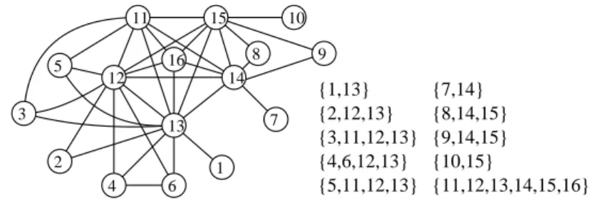
16 5 3 2 4 6 13 12 11 15 9 8 10 7 14 1 {3,11,12,13} {5,11,12,13} {2,12,13} {11,12,13,14,15,16} {4,6,12,13} {8,14,15} {9,14,15} {7,14} {10,15} {1,13}

Fig. 2. A ptolemaic graph G which produce the directed laminar tree in Fig. 1

corresponding node in T (C(G)) is uniquely determined by maximal cliques. Therefore, we can deﬁne a mapping from each vertex to the vertex set in C in T (C(G)): We denote by C(v) the clique C with v ∈ `(C). When we know whether C(v) is in M or L, we specify it by writing CM(v) or CL(v). An

example is given in Fig. 2 (all maximal cliques are also depicted); for the graph G in the ﬁgure, −→T (C(G)) is given in Fig. 1. We also note that from −

→

T (C(G)) with labels, we can reconstruct the original ptolemaic graph uniquely

up to isomorphism. That is, two ptolemaic graphs G1 and G2 are isomorphic

if and only if labeled −→T (C(G1)) is isomorphic to labeled −→T (C(G2)).

Intuitively, a clique laminar tree subdivides a clique tree of a chordal graph. For a chordal graph, maximal cliques are joined in a looser way in the sense that a clique tree for a chordal graph is not always uniquely determined up to isomorphism. The clique laminar tree subdivides the relationships between maximal cliques by using their laminar structure.

We can easily see the following properties of −→T (C(G)), and they are useful

from the algorithmic point of view:

Corollary 6 If G is a ptolemaic graph, we have the following: (1) For each

maximal clique M inM(G), `(M) consists of simplicial vertices in M. (2) The vertices in a maximal clique M in M(G) induce a maximal directed subtree of −→T (C(G)) rooted at the node M. (3) Each leaf in T (C(G)) corresponds to a maximal clique in M(G).

It is well known that a graph is chordal if and only if it is the intersection graph of subtrees of a tree. By Theorem 5, we obtain an intersection model for ptolemaic graphs as follows:

Corollary 7 Let −→T be any directed graph such that its underlying graph T is a tree. Let T be any set of subtrees −→Tv such that −→Tv consists of a node C

and all vertices reachable to C in −→T . Then the intersection graph over T is ptolemaic. On the other hand, for any ptolemaic graph, there exists such an intersection model.

(11)

PROOF. The directed clique laminar tree −→T (C(G)) is the base directed

graph of the intersection model. For each v ∈ V , we deﬁne the node C such that v ∈ `(C). By deﬁnition, a clique C0 contains v if and only if there is a directed path from the corresponding node C0 to the node C on−→T (C(G)). 2

3.2 A Linear Time Construction of Clique Laminar Trees

The main theorem in this section is the following:

Theorem 8 Given a ptolemaic graph G = (V, E), the directed clique laminar

tree −→T (C(G)) can be constructed in O(n + m) time.

We will make the directed clique laminar tree −→T (C(G)) by separating the

vertices in G into the vertex sets inC(G) = M(G) ∪ L(G).

We ﬁrst compute (and ﬁx) a perfect elimination ordering v1, v2, . . . , vn by the

LBFS. The outline of our algorithm is similar to the algorithm for constructing a clique tree for a given chordal graph due to Spinrad in [29]. For each vertex

vn, vn−1, . . . , v2, v1, we add it into the tree and update the tree. For the current

vertex vi, let vj := min{N>i(vi)}. Then, in Spinrad’s algorithm [29], there are

two cases to be considered: N>i(vi) = C(vj) or N>i(vi) ⊂ C(vj). The ﬁrst

case is simple; just add vi into C(vj). In the second case, Spinrad’s algorithm

adds a new maximal clique C(vi) that consists of N>i(vi)∪ {vi}. However, in

our algorithm, involved case analysis is required. For example, in the latter case, the algorithm has to handle three vertex sets; two maximal cliques{vi}∪

N>i(vi) and C(vj) together with one vertex set N>i(vi) shared by them. In this

case, intuitively, our algorithm makes three distinct sets CM with `(CM) =

{vi}, CL with `(CL) = N>i(vi), and C with `(C) = C(vj)\ N>i(vi), and adds

two arcs (CM, CL) and (C, CL); this means that vi is in CM = N>i(vi)∪ {vi},

C is a clique C(vj), and CL is the vertex set shared by CM and C. However,

our algorithm has to handle more complicated cases since the set C(vj) (and

hence N>i(vi)) can already be partitioned into some vertex sets.

In −→T (C(G)), each node C stores its label `(C). Hence each vertex in G

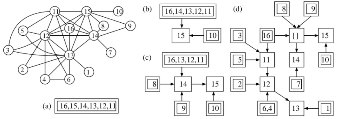
ap-pears exactly once in the tree. To represent it, each vertex v has a pointer to the node C(v) in C(G) = M(G) ∪ L(G). The detail of the algorithm is described as CliqueLaminarTree shown in Fig. 3, and an example of the construction is depicted in Fig. 4. In Fig. 4, the left-hand graph gives a ptolemaic graph (as same as Fig. 2), and the right-hand trees are clique lam-inar trees constructed (a) after adding the vertices 16, 15, 14, 13, 12, 11, (b) after adding the vertices 16, 15, 14, 13, 12, 11, 10, (c) after adding the vertices 16, 15, 14, 13, 12, 11, 10, 9, 8, and (d) after adding all the vertices. We show the correctness and a complexity analysis of the algorithm.

(12)

Fig. 3. Algorithm: CliqueLaminarTree

Input: A ptolemaic graph G = (V, E) with a PEO v1, v2, . . . , vn by the LBFS.

Output: A clique laminar tree T .

1: initialize T by the clique CM(vn) := {vn} and set the pointer from vn to CM(vn);

2: for i := n− 1 down to 1 do 3: let vj := min{N>i(vi)};

4: switch condition of N>i(vi) do

5: case (1) N>i(vi) = CM(vj)

6: update `(CM(vj)) := `(CM(vj))∪ {vi} and |CM(vj)| := |CM(vj)| + 1;

7: set CM(vi) := CM(vj);

8: case (2) N>i(vi) = CL(vj)

9: make a new maximal clique CM(vi) with `(CM(vi)) := {vi}

and |CM(vi)| := |CL(vj)| + 1;

10: add an arc (CM(vi), CL(vj));

11: case (3) N>i(vi)⊂ C(vj) and |`(C(vj))| = |C(vj)|

12: update `(C(vj)) := `(C(vj))\ N>i(vi)

and |`(C(vj))| := |`(C(vj))| − |N>i(vi)| ;

13: make a new vertex set L := N>i(vi) with `(L) := N>i(vi)

and |L| := |N>i(vi)| ;

14: make a new maximal clique CM(vi) with `(CM(vi)) = {vi}

and |CM(vi)| := |L| + 1;

15: add arcs (C(vj), L) and (CM(vi), L);

16: case (4) N>i(vi)⊂ C(vj) and |`(C(vj))| < |C(vj)|

17: make a new vertex set L := N>i(vi) with `(L) := N>i(vi)∩ `(C(vj))

and |L| := |N>i(vi)| ;

18: update `(C(vj)) := `(C(vj))\ L and |`(C(vj))| := |`(C(vj))| − |L| ;

19: make a new maximal clique CM(vi) with `(CM(vi)) = {vi}

and |CM(vi)| = |L| + 1;

20: remove the arc (C(vj), L0) with L0 ⊂ L and add an arc (L, L0);

21: add arcs (C(vj), L) and (CM(vi), L);

22: set the pointer from vi to C(vi);

23: return T . 16 5 3 2 4 6 13 12 11 15 9 8 10 7 14 1 16,15,14,13,12,11 16,14,13,12,11 15 10 16,13,12,11 15 10 9 14 16 12 6,4 9 11 {} 14 15 7 8 10 5 (a) (b) (c) (d) 3 2 13 1 8

(13)

We will use the following property of a PEO found by the LBFS of a chordal graph:

Lemma 9 ([9, Theorem 1]) Let v1, v2, . . . , vnbe a PEO found by the LBFS.

Then i < j implies max{N(vi)} ≤ max{N(vj)}.

This property is one of basic properties of LBFS, and hence the proof is omitted here. See Theorem 1 in [9], for example.

We assume that Algorithm CliqueLaminarTree is going to add vi, and let

vj := min{N>i(vi)}. We will show that all possible cases are listed, and in

each case, CliqueLaminarTree correctly manages the nodes in C(G) and their labels in O(deg(vi)) time. The following lemma drastically decreases the

number of possible cases and simpliﬁes the algorithm.

Lemma 10 Let vk be max{N>i(vi)}. In addition, assume that the set N>i(vi)

has already been divided into some distinct vertex sets L1, L2, . . . , Lh. Then,

there is an ordering of the sets such that vk∈ L1 ⊂ L2 ⊂ · · · ⊂ Lh.

PROOF. We ﬁrst observe that G[{vi, vi+1, . . . , vn}] is ptolemaic if G is

ptole-maic since any vertex induced subgraph of a chordal graph is chordal, and any vertex induced subgraph of a distance hereditary graph is distance hereditary. We assume that there is a vertex set L⊂ N>i(vi) such that L does not

con-tain vk. Then, there is a vertex vi0 with i0 > i that makes the vertex set L

before vi. Since {vi0, vk} 6∈ E, by Lemma 9, vi0 has another neighbor vk0 with

k0 > k. By the property of the LBFS, it is easy to see that G[{vk, . . . , vn}] is

connected. Let Mi be a maximal clique {vi} ∪ N>i(vi), and Mi0 be a maximal

clique that contains {vi0} ∪ L. Then, Mi∩ Mi0 = L which contains no vertex

in G[{vk, . . . , vn}]. On the other hand, we have {vi, vk}, {vi0, vk0} ∈ E. Hence,

Mi∩Mi0 does not separate Mi\Mi0 and Mi0\Mi. Therefore G[{vi, vi+1, . . . , vn}]

is not ptolemaic by Theorem 1(3), which is a contradiction. Thus we have

vk ∈ L, and hence, all the vertex sets L1, L2, . . . , Lh contain vk. The

ver-tex set N>i(vi) is contained in a maximal clique in the ptolemaic graph

G[{vi, vi+1, . . . , vn}]. Hence by Theorem 3, L1, L2, . . . , Lh are laminar.

There-fore, we have vk ∈ L1 ⊂ L2 ⊂ · · · ⊂ Lh for some appropriate ordering. 2

Proof of Theorem 8. Since the graph G is chordal and the vertices are

ordered in a perfect elimination ordering, N>i(vi) induces a clique. By Lemma

10, we have three possible cases; (a) N>i(vi) = C(vj), (b) N>i(vi) ⊂ C(vj)

and there are no vertex sets in N>i(vi), and (c) N>i(vi)⊂ C(vj) and there are

vertex sets L1 ⊂ L2 ⊂ · · · ⊂ Lh ⊂ N>i(vi). In the last case, we note that Lh 6=

N>i(vi); otherwise, we have vj ∈ Lh, or consequently, Lh = C(vj) = N>i(vi),

(14)

(a) N>i(vi) = C(vj): We have two subcases; C(vj) is a maximal clique

(i.e. N>i(vi) = CM(vj)) or C(vj) is a non-maximal clique (i.e. N>i(vi) =

CL(vj)). In the former case, we just update CM(vj) by CM(vj)∪ {vi}. This

is case (1) in CliqueLaminarTree. In the latter case, there is another ver-tex set that contains CL(vj) as a subset. Thus we add a new maximal clique

CL(vj)∪{vi}. More precisely, we add a new node CM(vi) with `(CM(vi)) ={vi}

and |CM(vi)| = |CL(vj)| + 1, and a new arc (CM(vi), CL(vj)). This is done

in case (2) of CliqueLaminarTree. We can check if N>i(vi) = C(vj) by

checking if |N>i(vi)| = |C(vj)| in O(1) time. Thus the time complexity is

O(1) in both cases.

(b) N>i(vi) ⊂ C(vj) and there are no vertex sets in N>i(vi): We

re-move N>i(vi) from C(vj) and make a new vertex set N>i(vi) shared by C(vj)

and CM(vi) = {vi} ∪ N>i(vj). We can observe that N>i(vi) ⊂ C(vj) and

there are no vertex sets in N>i(vi) if and only if |N>i(vi)| < |C(vj)| and

|`(C(vj))| = |C(vj)| . Thus, CliqueLaminarTree recognizes this case in

O(1) time, and handles it in case (3). It is easy to see that case (3) can be

done in O(|N>i(vi)| ) = O(deg(vi)) time. We note that, in this case, we do not

mind if C(vj) is maximal or not. In any case, the property does not change

for C(vj).

(c) N>i(vi) ⊂ C(vj) and there are vertex sets L1 ⊂ L2 ⊂ · · · ⊂ Lh ⊂

N>i(vi): We ﬁrst observe that the nodes Lh, Lh−1, . . . , L2, L1 with C(vj) form

a directed path (C(vj), Lh, . . . , L1) in−→T in the case. (Hence we can recognize

this case in O(|N>i(vi)| ) = O(deg(vi)) time, which will be used in Theorem

11.) Thus we make a new vertex set L := N>i(vi) with `(L) = N>i(vi)\ Lh.

The set N>i(vi)\Lhis given by N>i(vi)∩`(C(vj)). Then we update `(C(vj)) by

`(C(vj))\ N>i(vi). It is easy to add a maximal clique CM(vi) ={vi} ∪ N>i(vi).

Next, we have to update arcs around C(vj). By Lemma 10, this process is

simple; we can ﬁnd Lh in O(deg(vi)) time, and there is no other vertex set L0

that has an arc (C(vj), L0) which has to be updated. We note that there can

be some vertex set L0 with an arc (C(vj), L0). But L0 is independent from L

in this case, and hence we do not have to mind it. Finally, we change the arc (C(vj), Lh) to (L, Lh), and add the arcs (C(vj), L) and (CM(vi), L). Therefore

the time complexity in the last case is O(deg(vi)) time.

(15)

4 Applications of Clique Laminar Trees

4.1 The Recognition Problem

Theorem 11 The recognition problem for ptolemaic graphs can be solved in

linear time.

PROOF. Using the LBFS, we can obtain a perfect elimination ordering of G

in linear time if G is chordal (and reject it if G is not chordal). For a chordal graph, we run modiﬁed CliqueLaminarTree. It is not diﬃcult to modify CliqueLaminarTree to reject it if G is not distance hereditary. The key fact is that, if G is ptolemaic, N>i(vi) corresponds to a maximal directed path

in −→T (C(G)) as follows; suppose that we have vertex sets L1 ⊂ L2 ⊂ · · · ⊂

Lh ⊂ N>i(vi)⊂ C(vj) in case (c) in the proof of Theorem 8. In this case, (1)

the nodes form a connected directed path (C(vj), Lh, . . . , L2, L1) in −→T (C(G)),

(2) there are no other set L with L ⊂ L1, (3) all vertices in Lh (and hence

L1∪ L2∪ · · · ∪ Lh) belong to N>i(vi), and (4) some vertices in C(vj) may not

be in N>i(vi). Checking them can be done in O(|N>i(vi)| ) = O(deg(vi)) time

for each i, and otherwise, the vertex sets in the tree are not laminar, and hence they would be rejected. Cases (a) and (b) can be seen as special cases of case (c). Therefore, the total running time of the modiﬁed CliqueLaminarTree is still O(n + m). 2

We note that the result in Theorem 11 is not necessarily new. Since a graph is ptolemaic if and only if it is chordal and distance-hereditary [20], distance hereditary graphs are recognized in linear time [5,10,11,18], and chordal graphs are also recognized in linear time [28,31], we have Theorem 11 by combining them. We dare to state Theorem 11 to show that we can recognize if a graph is ptolemaic and then construct its clique laminar tree at the same time in linear time, and the algorithm is much simpler and more straightforward than the combination of known algorithms. (As noted in Introduction, the linear time algorithm for recognition of distance hereditary graphs is not so simple.)

4.2 The Graph Isomorphism Problem

Theorem 12 The graph isomorphism problem for ptolemaic graphs can be

(16)

PROOF. Given a ptolemaic graph G = (V, E), the labeled clique laminar

tree −→T (C(G)) is uniquely determined up to isomorphism: Maximal cliques

are uniquely determined, and so are M(G) and C(G). By Theorem 3, they form a laminar structure, and hence −→T (C(G)) is the unique tree structure

for given ptolemaic graph G by Lemma 2. Each vertex in V appears once in

−

→_{T (}_{C(G)), and the number of nodes in −}→_{T (}_{C(G)) is at most 2 |V | −1 by Lemma}

2(2). Thus the representation of −→T (C(G)) requires O( |V | ) space. The graph

isomorphism problem for labeled trees can be done in linear time (see, e.g., [25]), which completes the proof. 2

It is worth mentioning that the graph isomorphism problem can be solved in

O(n) time if a ptolemaic graph is given in the tree representation.

4.3 The Hamiltonian Cycle Problem

We assume that a ptolemaic graph G = (V, E) is given by a directed clique laminar tree −→T (C(G)) = (C(G), A(G)). Then the main theorem in this section

is the following:

Theorem 13 The Hamiltonian cycle problem for ptolemaic graphs can be

solved in O(n) time.

We remind that −→T (C(G)) takes O(n) space. We then remind that each clique C in C is a separator of G; removing C makes G disconnected. Hence, if −

→

T (C(G)) contains a vertex set C with |C| = 1, G does not have a Hamiltonian

cycle. This condition can be checked in O(n) time over −→T (C(G)). Therefore,

hereafter, we assume that any vertex set C in C satisﬁes |C| > 1.

Let L be a vertex set inC(G). We remind that the notions in ordinary trees are slightly abused on −→T (C(G)): A root has indegree 0, and a leaf has outdegree

0. That is, each maximal clique corresponds to a root. Note that a vertex set can have two or more parents when it is shared by some maximal cliques. We deﬁne ancestors and descendants as in ordinary trees. We regard any node L as an ancestor and descendant of itself. We denote by c(L) and p(L) the number of children of L and the number of parents of L in −→T (C(G)), respectively.

Hence p(M ) = 0 for each maximal clique M , and c(L) = 0 for each minimal vertex set L.

The basic idea to construct a Hamiltonian cycle is as follows. By Lemma 4, each clique L in −→T (C(G)) is a separator of its parents P1, . . . , Pk. Hence, to

visit all vertices, at least k edges in L has to be used to join the parents. More precisely, each edge will replaced by a path which visits all vertices in a parent

(17)

L M1

M2

M3

Fig. 5. Assignment of an edge to a path.

C C1 C2 C3 P1 P2

Fig. 6. Connection of children and par-ents.

and its ancestors. If L has enough vertices (and edges) in `(L), they can be used. However, if `(L) does not have enough resources, L has to use some edges which are in `(C) where C is a child or descendants of L. This observation also means that some parents may require two or more edges from `(L) to join their ancestors, and hence L and its descendants may have to provide more than k edges. Thus, we will say margin of L which is the number of edges in

L that ancestors can use. For an arc (P, L), a distribution is that the number

of edges L provides to P and its ancestors. In other words, we will consider

assignment of a path in L to each parent. We will say that L has feasible

distribution if the total distribution of arcs to L is less than or equal to the margin of L; that is, L and its descendants have enough edges to join their parents and ancestors. We give more detailed discussion below.

(i) We ﬁrst consider a minimal vertex set L with c(L) = 0. By Lemma 4, each L in L(G) is a separator of G. We can see that if we remove L from G, we have p(L) connected components. Hence, if |L| < p(L), G cannot have a Hamiltonian cycle. On the other hand, when |L| = p(L), any Hamiltonian cycle uses all vertices in L to connect each connected components. This fact can be seen as follows (Figure 5); we ﬁrst make a cycle of length |L| in L, and next replace each edge by a path through the vertices in one vertex set corresponding to a child of the node L. We then assign each edge to distinct parent of L. (When |L| = 2, we temporarily assign two (multi)edges.) If

|L| > p(L), we can construct a Hamiltonian cycle that uses |L| − p(L) edges

in G[L]. In this case, we need to assign p(L) edges in L to construct a cycle, and we also have |L| − p(L) edges which can be assigned in some other ancestors. We then deﬁne the margin m(L) by |L| − p(L) = |`(L)| − p(L). That is, if

m(L) < 0, G has no Hamiltonian cycle, and if m(L) > 0, we have extra m(L)

edges in L which can be assigned in some ancestors. We note that a margin can be inherited only from a descendant to an ancestor.

We here deﬁne a distribution δ((Cj, Ci)) of the margin, which is a function

assigned to each arc (Cj, Ci) ∈ −→T (C(G)). Let P1, . . . , Pp(L) be the parents of

(18)

∑p(L)

i=1 δ((Pi, L)) = m(L). That is, each parent Pi inherits δ((Pi, L)) margins

from L, and some ancestors of Pi will consume δ((Pi, L)) margins from L. The

way to compute the distribution will be discussed later.

(ii) We next consider a vertex set L with c(L) > 0 and p(L) ≥ 0, that is, L is a vertex set which is not minimal. Let C1, C2, . . . , Ch be children of L and

P1, P2, . . . , Pk parents of L in −→T (C(G)). That is, we have Ci ⊂ L ⊂ Pj for each

i and j with 1≤ i ≤ h = c(L) and 1 ≤ j ≤ k = p(L) (k = p(L) = 0 when L is

a maximal clique). We assume that m(Ci) and δ((L, Ci)) are already deﬁned

for each Ci, and m(Ci) ≥ 0 (otherwise G does not have any Hamiltonian

cycle). As in the ﬁrst case, we have to assign p(L) edges in L. In this case, each child Cican be used as a single vertex if δ((L, Ci)) = 0 (Figure 6); we ﬁrst

cut (remove) the assigned edge in Ci for L, and replace it by the path through

all vertices in L and its parents. If δ((L, Ci)) > 0 for some Ci, we can use the

additional vertices to connect parents Pj. Hence the margin m(L) is deﬁned

by |`(L)| + h +∑h_i=1δ((L, Ci))− k = |`(L)| +

∑_h

i=1(δ((L, Ci)) + 1)− k. The

distribution of the margin is deﬁned as the same as in the ﬁrst case; δ((Pi, L))

is a function such that ∑k_i=1δ((Pi, L)) = m(L).

The above discussion leads us to the following theorem:

Theorem 14 Let G = (V, E) be a ptolemaic graph. Then G has a

Hamilto-nian cycle if and only if there exist feasible distributions of margins, that is, each vertex set L in C satisfies m(L) ≥ 0.

We can see that the margin m(M ) for any maximal clique M is positive in case (2) since k = 0. In other words, every maximal clique M does not require any distribution of margins from its parents.

Our linear time algorithm, sayA, runs on T (G); A collects the leaves in T (G), computes the margins, and repeats this process by computing the margin of L such that all neighbors of L have been processed except exactly one neighbor. The precise procedure for each vertex set L is described as follows:

(1) When the vertex set L is a leaf of T (G), L is a maximal clique in G, and hence δ((L, C)) is set to 0, where C is the unique child of L.

(2) When L is not a leaf of T (G), let C1, C2, . . . , Ch be children of L in

− →

T (C(G)), P1, P2, . . . , Pk parents of L in −→T (C(G)), and X be the only

neigh-bor which is not processed. Without loss of generality, we assume that either

X = Ch or X = Pk. To simplify the notation, we deﬁne h0 = h− 1 and k0 = k

if X = Ch, and h0 = h and k0 = k− 1 if X = Pk. We have three subcases.

(a) If L is a maximal clique in G, or k = 0, L requires no distribution of margins. Hence, A assigns δ((L, X)) = 0 (since X ⊂ L).

(19)

11 4,5 {} 6,7 1,2,3 8 12 10 9 12 {} 13 9 10 11 8 13 4 6 1 2 3 5 7 15 14 16 14,15 16 {} d:1 m:1

Fig. 7. Deﬁnition of margins.

(b) If L is a minimal vertex set with k > 0, h = 0, we have X = Pk. Then A

ﬁrst computes m(L) = |`(L)| − k0. Then, for each i with i = 1, 2, . . . , k0, each parent Pi has been processed, and it requires distribution δ((Pi, L))

to L. Hence A computes δ0((X, L)) = m(L) −∑k_i=10 δ((Pi, L)) = |`(L)| −

∑_k0

i=1(δ((Pi, L)) + 1). If δ0((X, L)) < 0, G has no Hamiltonian cycles.

Other-wise, A sets δ((X, L)) := δ0((X, L)).

(c) When L is not a maximal clique with k > 0 and h > 0, A ﬁrst com-putes the margin m(L) = |`(L)| +∑h_i=10 (δ((L, Ci)) + 1)− k0. Next, A

dis-tributes the margin m(L) to the parents P1, . . . , Pk0 by computing δ0 :=

m(L)−∑k_i=10 δ((Pi, L)) = |`(L)| +

∑_h0

i=1(δ((L, Ci)) + 1)−

∑_k0

i=1(δ((Pi, L)) + 1).

The value δ0 indicates the margin that will be exchanged between L and X. If X = Pk, that is, (X, L) is the arc in −→T (C(G)), A distributes all margins

δ0 to X, or sets δ((X, L)) = δ0. The margin can be inherited from a child to a parent. Thus, in this case, if δ0 < 0, G has no Hamiltonian cycles. When δ0 ≥ 0, A will use the margin δ0 when it processes the vertex set X.

On the other hand, if X = Ch, that is, (L, X) is the arc in −→T (C(G)), the

margin will be distributed from X to L. Hence, if δ0 < 0, the vertex L borrows

margin δ0 from X which will be adjusted when the vertex X is chosen by A. ThusA sets δ((L, X)) = −δ0 in this case. If δ0 ≥ 0, the margin is useless since the child X only counts the number of its parents L, and does not use their margins. Therefore, δ((L, X)) will not be used, and hence A does nothing. (3) When L is the last node of the process; that is, every value of δ((L, L0)) for each neighbor L0 of L has been computed. Let C1, C2, . . . , Ch be children

of L in −→T (C(G)), and P1, P2, . . . , Pk be parents of L in −→T (C(G)). In this case,

A computes m(L) = |`(L)| +∑h

i=1(δ((L, Ci)) + 1)−

∑_k

i=1(δ((Pi, L)) + 1). If

m(L) < 0, L does not have enough margin. Hence G has no Hamiltonian cycle.

Otherwise, every node has enough margin, and hence G has a Hamiltonian cycle.

A simple example is depicted in Figure 7, where{1, 2, . . . , 7} induces a clique; the node L with `(L) ={1, 2, 3} has margin 1, and the arc from L0 to L with

(20)

L0 ={1, 2, 3, 4, 5} has distribution 1. The other nodes have margin 0, and the other arcs have distribution 0. Hence the graph in Figure 7 has a Hamiltonian cycle, e.g., (1, 8, 2, 9, 3, 10, 4, 11, 5, 14, 16, 15, 7, 12, 6, 13, 1).

The correctness of A can be proved by a simple induction for the number of nodes in −→T (C(G)) with Theorem 14. On the other hand, since T (G) contains O(n) nodes, the algorithm runs in O(n) time and space, which completes the

proof of Theorem 13. We note that the construction of a Hamiltonian cycle can be done simultaneously in O(n) time and space.

5 Concluding Remarks

In this paper, we present a new tree representation (data structure) for ptole-maic graphs. The result enables us to use the dynamic programming technique to solve some basic problems on this graph class. We presented a linear time algorithm for the Hamiltonian cycle problem, as one of such typical examples. To develop such eﬃcient algorithms based on the dynamic programming for other problems are future works.

We note that, recently, one of the authors and his colleagues extend the al-gorithm for the Hamiltonian cycle problem, and obtain a polynomial time algorithm for ﬁnding a longest cycle and path in a ptolemaic graph [30].

Acknowledgment

The authors are grateful to anonymous referees, who give numerous sugges-tions, and tell us the relationship between our results and those in relational database theory.

References

[1] H.-J. Bandelt and H.M. Mulder. Distance-Hereditary Graphs. Journal of Combinatorial Theory, Series B, 41:182–208, 1986.

[2] C. Beeri, R. Fagin, D. Maier, and M. Yannakakis. On the desirability of acyclic database schemes. Journal of the ACM, 30(3):479–513, 1983.

[3] A. Brandst¨adt and F.F. Dragan. A Linear-Time Algorithm for Connected

r-Domination and Steiner Tree on Distance-Hereditary Graphs. Networks,

(21)

[4] A. Brandst¨adt, V.B. Le, and J.P. Spinrad. Graph Classes: A Survey. SIAM Monographs on Discrete Math. and Appl., Vol. 3, 1999.

[5] A. Bretscher, D. Corneil, M. Habib, and C. Paul. A Simple Linear Time LexBFS Cograph Recognition Algorithm. In Graph-Theoretic Concepts in

Computer Science (WG 2003), pages 119–130. Lecture Notes in Computer

Science Vol. 2880, Springer-Verlag, 2003.

[6] H.J. Broersma, E. Dahlhaus, and T. Kloks. A linear time algorithm for minimum ﬁll-in and treewidth for distance hereditary graphs. Discrete Applied

Mathematics, 99:367–400, 2000.

[7] M.-S. Chang, S.-Y. Hsieh, and G.-H. Chen. Dynamic Programming on Distance-Hereditary Graphs. In Proceedings of 8th International Symposium

on Algorithms and Computation (ISAAC ’97), pages 344–353. Lecture Notes in

Computer Science Vol. 1350, Springer-Verlag, 1997.

[8] M.-S. Chang, S.-C. Wu, G.J. Chang, and H.-G. Yeh. Domination in distance-hereditary graphs. Discrete Applied Mathematics, 116:103–113, 2002.

[9] D.G. Corneil. Lexicographic Breadth First Search — A Survey. In

Graph-Theoretic Concepts in Computer Science (WG 2004), pages 1–19. Lecture Notes

in Computer Science Vol. 3353, Springer-Verlag, 2004.

[10] D.G. Corneil, Y. Perl, and L.K. Stewart. A Linear Recognition Algorithm for Cographs. SIAM Journal on Computing, 14(4):926–934, 1985.

[11] G. Damiand, M. Habib, and C. Paul. A Simple Paradigm for Graph Recognition: Application to Cographs and Distance Hereditary Graphs.

Theoretical Computer Science, 263:99–111, 2001.

[12] A. D’Atri and M. Moscarini. Distance-Hereditary Graphs, Steiner Trees, and Connected Domination. SIAM Journal on Computing, 17(3):521–538, 1988. [13] A. D’Atri and M. Moscarini. On Hypergraph Acyclicity and Graph Chordality.

Information Processing Letters, 29:271–274, 1988.

[14] R. Fagin. Degrees of Acyclicity for Hypergraphs and Relational Database Schemes. Journal of the ACM, 30(3):514–550, 1983.

[15] M. Farber. Independent Domination in Chordal Graphs. Operations Research

Letters, 1(4):134–138, 1982.

[16] F. Gavril. Algorithms for Minimum Coloring, Maximum Clique, Minimum Covering by Cliques, and Maximum Independent Set of a Chordal Graph. SIAM

Journal on Computing, 1(2):180–187, 1972.

[17] M.C. Golumbic. Algorithmic Graph Theory and Perfect Graphs. Annals of Discrete Mathematics 57. Elsevier, 2nd edition, 2004.

[18] P.L. Hammer and F. Maﬀray. Completely Separable Graphs. Discrete Applied

(22)

[19] E. Howorka. A Characterization of Distance-Hereditary Graphs. Quart. J.

Math. Oxford (2), 28:417–420, 1977.

[20] E. Howorka. A Characterization of Ptolemaic Graphs. Journal of Graph Theory, 5:323–331, 1981.

[21] S.-Y. Hsieh, C.-W. Ho, T.-S. Hsu, and M.-T. Ko. The Hamiltonian Problem on distance-hereditary graphs. Discrete Applied Mathematics, 154:508–524, 2006. [22] R.-W. Hung and M.-S. Chang. Linear-time algorithms for the Hamiltonian

problems on distance-hereditary graphs. Theoretical Computer Science,

341:411–440, 2005.

[23] S. i. Nakano, R. Uehara, and T. Uno. A New Approach to Graph Recognition and Applications to Distance Hereditary Graphs. In 4th Annual Conference on

Theory and Applications of Models of Computation (TAMC 07), pages 115–127.

Lecture Notes in Computer Science Vol. 4484, Springer-Verlag, 2007.

[24] P.N. Klein. Eﬃcient Parallel Algorithms for Chordal Graphs. SIAM Journal

on Computing, 25(4):797–827, 1996.

[25] J. K¨obler, U. Sch¨oning, and J. Tor´an. The Graph Isomorphism Problem: Its

Structural Complexity. Birkh¨auser, 1993.

[26] B. Korte and J. Vygen. Combinatorial Optimization, volume 21 of Algorithms

and Combinatorics. Springer, 2000.

[27] F. Nicolai and T. Szymczak. Homogeneous Sets and Domination: A Linear Time Algorithm for Distance-Hereditary Graphs. Networks, 37(3):117–128, 2001. [28] D.J. Rose, R.E. Tarjan, and G.S. Lueker. Algorithmic Aspects of Vertex

Elimination on Graphs. SIAM Journal on Computing, 5(2):266–283, 1976. [29] J.P. Spinrad. Eﬃcient Graph Representations. American Mathematical Society,

2003.

[30] Y. Takahara, S. Teramoto, and R. Uehara. Longest Path Problems on Ptolemaic Graphs. IEICE Transactions, E91-D(2):170–177, 2008.

[31] R.E. Tarjan and M. Yannakakis. Simple Linear-Time Algorithms to Test Chordality of Graphs, Test Acyclicity of Hypergraphs, and Selectively Reduce Acyclic Hypergraphs. SIAM Journal on Computing, 13(3):566–579, 1984. [32] R. Uehara and Y. Uno. Laminar Structure of Ptolemaic Graphs and Its

Applications. In 16th Annual International Symposium on Algorithms and

Computation (ISAAC 2005), pages 186–195. Lecture Notes in Computer Science

Vol. 3827, Springer-Verlag, 2005.

[33] H.-G. Yeh and G.J. Chang. Centers and medians of distance-hereditary graphs.