Weak solvability
for
abstract
nonlinear
Schr\"odinger
equations
東京理科大学大学院理学研究科D3 鈴木敏行 (Toshiyuki Suzuki)
Department ofMathematics, Tokyo University of Science
1. Introduction
In this paper we consider the following Cauchy problem for nonlinear Schr\"odinger
equations with inverse-square potential:
$(CP)_{a}$ $\{\begin{array}{ll}i\frac{\partial u}{\partial t}=(-\Delta+\frac{a}{|x|^{2}})u+f(u) in \mathbb{R}\cross \mathbb{R}^{N},u(O, x)=u_{0}(x) on \mathbb{R}^{N},\end{array}$
where $i=\sqrt{-1},$ $a>-(N-2)^{2}/4$
.
The feature for $(CP)_{a}$ is the presence ofa stronglysingular potential $a|x|^{-2}$; note that $-\Delta$ and $a|x|^{-2}$ are the samescale symmetry:
$(-\Delta)[u(\lambda x)]=\lambda^{2}(-\Delta u)(\lambda x) , (|x|^{-2})[u(\lambda x)]=\lambda^{2}(|\cdot|^{-2}u)(\lambda x) , \forall\lambda>0.$
This implies that the so-called scaling argument
can
not be applied to$P_{a}:=- \Delta+\frac{a}{|x|^{2}}.$
Inother words, $(CP)_{a}$
can
not be reduced to thecase
with $|a|$ and $\Vert u_{0}\Vert_{H^{1}}$ small enough.On the other hand, from the viewpoint of operator theory, $P_{a}=-\triangle+a|x|^{-2}$ is
nonnegative and selfadjoint in $L^{2}(\mathbb{R}^{N})$ (as form-sum) if $N\geq 3$ and $a\geq-(N-2)^{2}/4.$
Moreover, $P_{a}$ is nonnegative and selfadjoint in $H^{-1}(\mathbb{R}^{N})$ with domain $D(P_{a})=H^{1}(\mathbb{R}^{N})$
if$N\geq 3$ and $a>-(N-2)^{2}/4$
.
These are consequences of the Hardy inequality$\frac{N-2}{2}\Vert\frac{u}{|x|}\Vert_{L^{2}}\leq\Vert\nabla u\Vert_{L^{2}} \forall u\in H^{1}(\mathbb{R}^{N}), N\geq 3.$
If$f(u)\equiv 0$ and $u_{0}\in H^{1}(\mathbb{R}^{N})$, then $e^{-itP_{a}}u_{0}$ is a unique solution to $(CP)_{a}$ in $H^{-1}(\mathbb{R}^{N})$
.
Now we consider $f(u)\not\equiv 0$. If $V\in L^{\infty}(\mathbb{R}^{N})+L^{p}(\mathbb{R}^{N})$ for some $p\geq N/2$, then
$V(x)u+f(u)$ can be regarded
as a
nonlinear term. For example, let $V(x)$ $:=|x|^{-\alpha}$$(\alpha>0)$
.
Then $V\in L^{\infty}(\mathbb{R}^{N})+L^{p}(\mathbb{R}^{N})$ for all $p<N/\alpha$. In paticular, if$0<\alpha<2$, then $|x|^{-\alpha}\in L^{\infty}(\mathbb{R}^{N})+L^{N/2}(\mathbb{R}^{N})$.
However, $V(x)=|x|^{-2}\not\in L^{\infty}(\mathbb{R}^{N})+If(\mathbb{R}^{N})(\alpha=2)$ forany$p\geq N/2$. Hencewe cannot regard the term$a|x|^{-2}u$ as apartof the nonlinearterm.
Theabove considerationsuggeststhatwemayapplytheprecedingmethodsto $(CP)_{a}$
by replacing -$A$ with $P_{a}$. However, there exist a lot of difficulties for solving $(CP)_{a}$
by the preceding methods: Ginibre-Velo’s[6], Kato’s[8], Cazenave-Weissler’s[5] and
Cazenave’s[3, 4].
(i) There is no work for the dispersiveestimates for $e^{-itP_{a}}$:
where$P_{a}$ $:=-\triangle+a|x|^{-2}$. Hence wecannot apply Ginibre-Velo’s method [6, 7] because
$L^{q}-L^{q’}$ type estimates is essentially
used;
(ii) We can apply Kato’s method [8] since the Strichartz estimates are available in [1]:
$\Vert e^{-itP_{a}}u_{0}\Vert_{L^{\tau}(\mathbb{R};L\rho(\mathbb{R}^{N}))}\leq C\Vert u_{0}\Vert_{L^{2}(\mathbb{R}^{N})}, \frac{2}{\tau}+\frac{N}{\rho}=\frac{N}{2}, \tau, \rho\geq 2.$
Applying Kato’s method, Okazawa, Suzuki and Yokota[10] showed the following fact:
define $f(u)$ $:=\lambda|u|^{p-1}u$, where $\lambda$ and
$p$ satisfies $1\leq p<(N+2)/(N-2)(\lambda>0)$ or
$1\leq p<1+4/N(\lambda<0)$
.
Assume(1.1) $a>[ \frac{N(p-1)}{2(p+1)}]^{2}-\frac{(N-2)^{2}}{4}.$
Then for every $u_{0}\in H^{1}(\mathbb{R}^{N})$ there exists a uniqueglobal weak solution $u$ to $(CP)_{a}$. To
establish thisfact we evaluate $\Vert\nabla u\Vert_{L^{\tau}(I;L^{p}(\mathbb{R}^{N}))}$. Since $\nabla$ and$e^{-itP_{a}}$ arenot commutative,
we use the following Strichartz type estimates:
$\Vert\nabla e^{-itP_{a}}u_{0}\Vert_{L^{\tau}(\mathbb{R};L^{p}(\mathbb{R}^{N}))}\leq C\Vert\nabla u_{0}\Vert_{L^{2}(\mathbb{R}^{N})} [a+(N-2)^{2}/4]^{1/2}>2/\tau.$
To construct local weak solutions we choose
$(\tau, \rho)=(\infty, 2)$ and $( \tau, \rho)=(\frac{4(p+1)}{N(p-1)},p+1)$.
The latter pair applies to give the unsatisfactory restriction (1.1) on $a.$
(iii) Cazenave-Weissler[5] and Cazenave[4, Chapter 3] developed other methods. But
those are not applicable to the critical case $(for$ example, $f(u)$ $:=(W*|u|^{2})u$ for $W\in$
$L^{N/4}(\mathbb{R}^{N}))$; this critical case canbe dealt with Ginibre-Velo[7] when $a=0.$
(iv) Cazenave’s method [4, Chapter 3] is useful becausesolvability of $(CP)_{a}$ with$a=0$
is verified without either the dispersive estimates or the Strichartz estimates. But his
method uses the $m$-accretivity $of-\triangle$ in $L^{q}(\mathbb{R}^{N})$. Here $P_{a}=-\triangle+a|x|^{-2}$ does not seem
to be $m$-accretive in $L^{q}(\mathbb{R}^{N})$ if $a$ is near to $-(N-2)^{2}/4$. More precisely, Okazawa [9]
proved the $m$-accretivity of$P_{a}$ in$L^{q}(\mathbb{R}^{N})$ with
$a>\{\begin{array}{ll}\frac{(q-1)(2q-N)N}{q^{2}}, q\in[\frac{2(N-1)}{N}, \infty) ,(q-1)(N-2)^{2} -\overline{q^{2}}, q\in[1, \frac{2(N-1)}{N}].\end{array}$
The lower bounds of$a$ is greater than $-(N-2)^{2}/4$ if$q\neq 2.$
Thus we need another new approach to solve $(CP)_{a}$. In Section 2 we introduce
energy methods for abstract nonlinear Schr\"odinger equations. Application to $(CP)_{a}$
with power type nonlinearityis stated in Section 3. Application to $(CP)_{a}$ withnonlocal
nonlinearity (Hartree type equations) is given in Section 4. Section 5 is devoted to the
proofof the solvability of Hartree typeequations inSection 4. Finally, some remarks are
2.
Abstract theory for nonlinear
Schr\"odinger
equations
Let $S$ be a nonnegative selfadjoint operator in a complex Hilbert space $X$
.
Put$X_{S}$ $:=D(s^{1/2})$. Then we have the usual triplet: $X_{S}\subset X=X^{*}\subset X_{S}^{*}$
.
Under thissetting$S$
can
be extended to anonnegative selfadjoint operator in $X_{S}^{*}$ with domain $X_{\mathcal{S}}.$Now we consider
(ACP) $\{\begin{array}{l}i\frac{du}{dt}=Su+g(u) ,u(0)=u_{0},\end{array}$
where $g:X_{S}arrow X_{S}^{*}$ is a nonlinear operator satisfying
(Gl) Existence ofenergy functional: there exists $G\in C^{1}(X_{S};\mathbb{R})$ such that $G’=g,$
that is, given $u\in X_{S}$, for every $\epsilon>0$ there exists $\delta=\delta(u, \epsilon)>0$ such that
$|G(u+v)-G(u)-{\rm Re}\langle g(u),$$v\rangle_{X_{S}^{*},X_{S}}|\leq\epsilon\Vert v\Vert_{X_{\mathcal{S}}}$ $\forall v\in X_{S}$ with $\Vert v\Vert_{X_{S}}<\delta$;
(G2) Local Lipschitz continuity: for all $M>0$ there exists $C(M)>0$ such that
$\Vert g(u)-g(v)\Vert_{X_{\dot{S}}}\leq C(M)\Vert u-v\Vert_{X_{S}}$ $\forall u,$ $v\in X_{S}$ with $\Vert u\Vert_{X_{S}},$ $\Vert v\Vert_{X_{S}}\leq M$;
(G3) H\"older-like continuity of
energy
functional: given $M>0$, forall $\delta>0$ thereexists a constant $C_{\delta}(M)>0$ such that
$|G(u)-G(v)|\leq\delta+C_{\delta}(M)\Vert u-v\Vert_{X}$ $\forall u,$ $v\in X_{S}$with $\Vert u\Vert_{X_{S}},$ $\Vert v\Vert_{X_{S}}\leq M$;
(G4) Gauge type condition for the conservation of charge:
${\rm Im}\langle g(u), u\rangle_{X_{\dot{\mathcal{S}}},X_{S}}=0 \forall u\in X_{S}$;
(G5) Closedness type condition: given a bounded open interval $I\subset \mathbb{R}$, let $\{w_{n}\}_{n}$
be any bounded sequence in $L^{\infty}(I;X_{S})$ such that
(2.1) $\{\begin{array}{ll}w_{n}(t)arrow w(t)(narrow\infty) weakly in X_{S} a.a.t\in I,g(w_{n})arrow f(narrow\infty) weakly^{*} in L^{\infty}(I;X_{S}^{*}) .\end{array}$
Then
(2.2) ${\rm Im} l\langle f(t), w(t)\rangle_{X_{S}^{*},X_{S}}dt=narrow\infty hm{\rm Im}l\langle g(w_{n}(t)), w_{n}(t)\rangle_{X_{S}^{*},X_{S}}dt.$
Here $f=g(w)$ is guaranteed if
(2.3) $w_{n}(t)arrow w(t)(narrow\infty)$ strongly in$X$ a.a. $t\in I$;
(G6) Lower boundedness of the energy: there exist $\epsilon\in(0,1] and C_{0}(\cdot)\geq 0$ such
that
$G(u) \geq-\frac{1-\epsilon}{2}\Vert u\Vert_{X_{S}}^{2}-C_{0}(\Vert u\Vert_{X}) \forall u\in X_{S}.$
Here a function $u$ is said to be a local weak solution on $I$ to (ACP) if$u$ belongs
to$L^{\infty}(I;X_{S})\cap W^{1,\infty}(I;X_{S}^{*})_{\mathfrak{U}1}d$ satisfies (ACP) in $L^{\infty}(I;X_{S}^{*})$
.
If $I$ coincides with$\mathbb{R},$Theorem 2.1 (Local existence, [11]). Assume that$g:X_{S}arrow X_{S}^{*}satisf\iota’es$ (Gl)$-(G5)$
.
Then
for
every $u_{0}\in X_{S}$ with $\Vert u_{0}\Vert_{x_{s}}\leq M$ there exist$T_{M}>0$ and a local weak solutionon $(-T_{M}, T_{M})$
.
Moreover$\Vert u(t)\Vert_{X}=\Vert u_{0}\Vert_{X}, E(u(t))\leq E(u_{0}) \forall t\in[-T_{M}, T_{M}],$ where $E(\cdot)$ is the energygiven by$E(\varphi):=(1/2)\Vert s^{1/2_{\varphi\Vert_{X}^{2}}}+G(\varphi),$ $\varphi\in X_{S}.$
Proof of Theorem 2.1 is based on Cazenave’s method. But we avoid to apply $Iy$
theory to the nonnegative selfadjoint operator $S$. Now we give a sketch of the proof of
Theorem 2.1.
Proofof Theorem 2.1 (Step 1). We consider the approximate problems in$X$:
$(ACP)_{\epsilon}$ $\{\begin{array}{l}i\frac{du_{\epsilon}}{dt}=Su_{\epsilon}+g_{\epsilon}(u_{\epsilon}) ,u_{\epsilon}(0)=u_{0},\end{array}$
where $g_{\epsilon}$ is the approximation of
$g$ defined as
$g_{\epsilon}(u):=(1+\epsilon S)^{-1/2}g((1+\epsilon S)^{-1/2}u)$
Note that $g_{\epsilon}$ is locally Lipschitz continuous on $X.$
By virtue of (Gl), (G2) and (G4), $($ACP$)_{\epsilon}$ admits aunique global weak solution
$u_{\epsilon}$ belonging to $C(\mathbb{R};X_{S})\cap C^{1}(\mathbb{R};X_{S}^{*})$
.
More precisely, we apply the following theoremto $g_{0}(u):=g_{\epsilon}(u)$ and $G_{0}(u):=G((1+\epsilon S)^{-1/2}u)$.
Proposition 2.2 ([4, Theorem 3.3.1]). Let $S:X_{S}\subset X_{S}^{*}arrow X_{S}^{*}$ be a nonnegative
selfadjoint opemtor. Assume that $g_{0}:Xarrow X$
satisfies
(i) there exists $G_{0}\in C^{1}(X_{S};\mathbb{R})$ such that$G_{0}’=g_{0}$, thatis, given$u\in X_{S}$,
for
every$\epsilon>0$there $ex!ists\delta=\delta(u,\epsilon)>0$ such that
$|G_{0}(u+v)-G_{0}(u)-{\rm Re}\langle g_{0}(u),$$v\rangle_{X}|\leq\epsilon\Vert v\Vert_{X_{S}}$ $\forall v\in X_{S}$ with$\Vert v\Vert_{X_{\mathcal{S}}}<\delta$;
(ii) $g_{0}$ is locally Lipschitz continuous on $X$:
$\Vert g_{0}(x)-g_{0}(y)\Vert_{X}\leq L(M)\Vert x-y\Vert_{X}$ $\forall x,$ $y\in X$ with $\Vert x\Vert_{X},$ $\Vert y\Vert_{X}\leq M$; (iii) ${\rm Re}\langle g_{0}(u),$$iu\rangle_{X}=0\forall u\in X.$
Then
for
evew
$x\in X_{S}$ there exists a unique solution $u\in C(\mathbb{R};X_{S})\cap C^{1}(\mathbb{R};X_{s}^{*})$ to$\{\begin{array}{l}i\frac{du}{dt}=Su+g_{0}(u) in \mathbb{R},u(0)=x,\end{array}$
Moreover conservation laws hold:
$\Vert u(t)\Vert_{X}=\Vert x\Vert_{X}, E_{0}(u(t))=E_{0}(x) \forall t\in \mathbb{R},$
Proof of Theorem 2.1 (Step 2). We prove the uniform boundedness with respect to
$\epsilon>0$:
$\Vert u_{\epsilon}(t)\Vert_{X_{S}}\leq M’ \forall t\in[-T_{M}, T_{M}].$
This fact is proved in a way similar to Cazenave’s method. See [11, Lemma 4.2] (or [4,
Theorem 3.3.5]$)$
.
Proof of Theorem 2.1 (Step 3). Since $\Vert u_{\epsilon}(t)\Vert_{X_{S}}$and $\Vert u_{\epsilon}’(t)\Vert_{X_{\mathcal{S}}^{*}}$areuniformlybounded
in $[-T_{M}, T_{M}]$, the Ascoli type lemma (see [4, Proposition 1.1.2]) yields that there exist a sequence $\{u_{\epsilon_{k}}\}_{k}\subset\{u_{\epsilon}\}_{\epsilon}$ and a function $u\in C_{w}([-T_{M}, T_{M}];X_{S})\cap W^{1,\infty}(-T_{M}, T_{M};X_{S}^{*})$
such that
(2.4) $u_{\epsilon_{k}}(t)arrow u(t)(karrow\infty)$ weakly in $X_{S}$ $\forall t\in[-T_{M}, T_{M}].$
Hence it follows from $u_{\epsilon_{k}}’arrow u’(karrow\infty)weakly^{*}$in $L^{\infty}(-T_{M}, T_{M};X_{S}^{*})$ that $u$ satisfies
(ACP)’ $\{\begin{array}{l}i\frac{du}{dt}=Su+f in L^{\infty}(-T_{M}, T_{M};X_{S}^{*}) ,u(0)=u_{0}.\end{array}$
It suffices to show tfiat $f=g(u)$. To end this, we suppose weak closedness condition
(G5). In fact, since (2.4) and
$g((1+\epsilon_{k}S)^{-1/2}u_{\epsilon_{k}})arrow f(karrow\infty)$ $weakly^{*}$ in$L^{\infty}(-T_{M}, T_{M};X_{S}^{*})$,
(G5) and (G4) imply that
$\frac{1}{2}\Vert u(t)\Vert_{X}^{2}-\frac{1}{2}\Vert u_{0}\Vert_{X}^{2}={\rm Im}\int_{0}^{t}\langle f(s), u(s)\rangle_{X_{\dot{S}},X_{S}}ds=0$
This is nothing but the conservation law of charge. (2.4) and $\Vert u_{\epsilon_{k}}(t)\Vert_{X}=\Vert u_{0}\Vert_{X}=$
$\Vert u(t)\Vert_{X}$ yield that $u_{\epsilon_{k}}(t)arrow u(t)(karrow\infty)$ strongly in $X$
.
Hencewe see
from (G5) that$f=g(u)$
.
Therefore we have proved Theorem 2.1.
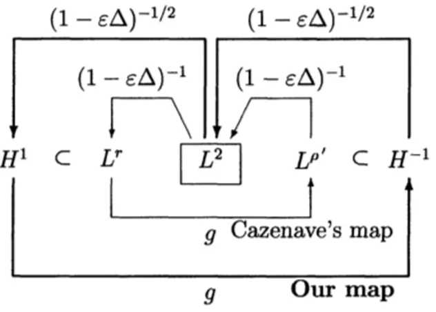
Here we compare Cazenave’s method with
ours
(see Figure 1). First wecan
makemore moderate approximation. Cazenave used the $m$-accretivity of-$A$ in If$(\mathbb{R}^{N})$ and
that the resolvent $(1-\epsilon\Delta)^{-1}$ maps from $L^{2}(\mathbb{R}^{N})$ to $L^{r}(\mathbb{R}^{N})(2\leq r<2N/(N-2))$ and
from $L^{\rho’}(\mathbb{R}^{N})(2\leq\rho<2N/(N-2))$to $L^{2}(\mathbb{R}^{N})$
.
Here $r=2N/(N-2)=\rho$ is excludedbecause he applied Rellich’s compactness theorem to verifying $f=g(u)$ in Step 3. We
do not need to apply Relhch’s compactness theorem by virtue of (G5).
Next we introduce the global existence of weak solutions to (ACP). Note that we need the uniqueness of local weak solution to (ACP).
Theorem 2.3 (Global existence, [11, Theorem2.4]). Assume that$g:X_{S}arrow X_{S}^{*}$
satisfies
(Gl)$-(G6)$ and the uniqueness
of
local weak solutions to (ACP). Thenfor
every $u_{0}\in$ $X_{S}$ there exists a global weak solution $u\in C(\mathbb{R};X_{S})\cap C^{1}(\mathbb{R};X_{S}^{*})$ to (ACP) and theconservation laws hold:
$g$ Our map
Figure 1: Comparison of Cazenave’s composite mapping and ours
3. Solvability
for
nonlinear
Schr\"odinger
equations of power type
We can apply Theorem 2.3 to $(CP)_{a}$ with power type nonlinearity. Assume that
$f$ : $\mathbb{C}arrow \mathbb{C}$ satisfies
(Nl) $f(0)=0$;
(N2) There exist $p\in[1, (N+2)/(N-2))$ and $K\geq 0$ such that
(3.1) $|f(u)-f(v)|\leq K(1+|u|^{p-1}+|v|^{p-1})|u-v| \forall u, v\in \mathbb{C}$;
(N3) $f(x)\in \mathbb{R}(x>0)$ and $f(e^{i\theta}z)=e^{i\theta}f(z)(z\in \mathbb{C}, \theta\in \mathbb{R})$;
(N4) There exist $q\in[1,1+4/N)$ and $L_{1},$$L_{2}\geq 0$ such that
(3.2) $F(x) := \int_{0}^{x}f(s)ds\geq-L_{1}x^{2}-L_{2}x^{q+1} \forall x>0.$
The conditions (Nl)$-(N4)$ are nothing but what was imposed by Ginibre-Velo [6] and
Kato [8]. Typical example of (Nl)$-(N4)$ is $f(u);=\lambda|u|^{p-1}u$ with
(i) $\lambda>0$ and $1\leq p<(N+2)/(N-2)$; (ii) $\lambda<0$ and $1\leq p<1+4/N.$
ApplyingTheorem 2.3, we obtain
Theorem 3.1 ([11, Theorem 5.1]). Let $N\geq 3,$ $a>-(N-2)^{2}/4$
.
Assume $f$ : $\mathbb{C}arrow$$\mathbb{C}$
satisfies
(Nl)$-(N4)$.
Thenfor
all $u_{0}\in H^{1}(\mathbb{R}^{N})$ there exists a unique global weaksolution to $(CP)_{a}$
.
Moreover, $u$ belongs to$C(\mathbb{R};H^{1}(\mathbb{R}^{N}))\cap C^{1}(\mathbb{R};H^{-1}(\mathbb{R}^{N}))$ andsatisfies
conserwation laws
$\Vert u(t)\Vert_{L^{2}}=\Vert u_{0}\Vert_{L^{2}}, E(u(t))=E(u_{0}) \forall t\in\mathbb{R},$
where the $l$
‘energy” is
defined
as$E( \varphi):=\frac{1}{2}\Vert\nabla\varphi\Vert_{L^{2}}^{2}+\frac{a}{2}\Vert\frac{\varphi}{|x|}\Vert_{L^{2}}^{2}+\int_{\mathbb{R}^{N}}\int_{0}^{|\varphi(x)|}f(s)d_{\mathcal{S}}.$
4. Solvability for Hartree type
equations
Next we consider the following problem:
$(HE)_{a}$ $\{\begin{array}{ll}i\frac{\partial u}{\partial t}=(-\Delta+\frac{a}{|x|^{2}})u+K(|u|^{2})u in \mathbb{R}\cross \mathbb{R}^{N},u(O, x)=u_{0}(x) on \mathbb{R}^{N},\end{array}$
where $K$ is
an
integral operator:(4.1) $K(f)(x)=Kf(x):= \int_{R^{N}}k(x,y)f(y)dy.$
The feature for $(HE)_{a}$ is the nonlocal nonlinearities $K(|u|^{2})u$
.
Let $a=0$ and $k(x, y)=$$W(x-y)$
.
Then $(HE)_{a}$ isthe usual Hartree equation (see [7]).We consider the kemel $k$ of the integral operator $K$ [defined by (4.1)].
Definition 4.1. $L_{x}^{\beta}(L_{y}^{\alpha})=L_{x}^{\beta}(\mathbb{R}^{N};L_{y}^{\alpha}(\mathbb{R}^{N}))$ is the family of$k:\mathbb{R}^{N}\cross \mathbb{R}^{N}arrow \mathbb{R}$ such that
(4.2) $\Vert k\Vert_{L_{x}^{\beta}(L_{y}^{\alpha})} =(\int_{\mathbb{R}^{N}}(\int_{\mathbb{R}^{N}}|k(x,y)|^{\alpha}dy)^{\beta/\alpha}dx)^{1/\beta}<\infty.$
Nowwe assume that the kemel $k$ satisfies the following three conditions:
(Kl) $k$ isasymmetric real-valuedfunction, thatis, $k(x, y)=k(y, x)\in \mathbb{R}$a.a.
$x,$ $y\in \mathbb{R}^{N}$;
(K2) $k\in L_{y}^{\infty}(L_{x}^{\infty})+L_{y}^{\beta}(L_{x}^{\alpha})$and $k-k_{R}arrow 0$in $L_{y}^{\beta}(L_{x}^{\alpha})$ forsome $\alpha,$ $\beta\in[1, \infty]$ such that
$\alpha\leq\beta,$ $\alpha^{-1}+\beta^{-1}\leq 4/N$;
(K3) $k_{-};=- \min\{k, 0\}\in L_{y}^{\infty}(L_{x}^{\infty})+L_{y}^{\tilde{\beta}}(L_{x}^{\tilde{\alpha}})$ and $k_{-}-(k_{-})_{R}arrow 0$ in $L_{y}^{\tilde{\beta}}(L_{x}^{\tilde{\alpha}})$ for
some
$\tilde{\alpha},\tilde{\beta}\in[1, \infty]$ such that $\tilde{\alpha}\leq\tilde{\beta},\tilde{\alpha}^{-1}+\tilde{\beta}^{-1}\leq 2/N.$
Here $k_{R}$ is defined as
(4.3) $k_{R}(x, y):=\{\begin{array}{l}k(x,y) |k(x,y)|\leq R,R k(x,y)>R,-R k(x,y)<-R.\end{array}$
For example, let $W\in If(\mathbb{R}^{N})$
.
Then $k(x,y)$ $:=W(x-y)$ belongs to $L_{x}^{\infty}(If_{y})$ andsatisfies $\Vert k\Vert_{L_{x}^{\infty}(L_{y}^{p})}=\Vert W\Vert_{L^{p}}.$
Theorem 4.1 ([13, Theorem 1.3]). Let $N\geq 3$ and $a>-(N-2)^{2}/4$
.
Assume that$k$
satisfies
(Kl)$-(K3)$.
Thenfor
every $u_{0}\in H^{1}(\mathbb{R}^{N})$ there enists a unique global weaksolution $u$ to $(HE)_{a}$
.
Moreover, $u$ belongs to $C(\mathbb{R};H^{1}(\mathbb{R}^{N}))\cap C^{1}(\mathbb{R};H^{-1}(\mathbb{R}^{N}))$ andsatisfies
conservation laws(4.4) $\Vert u(t)\Vert_{L^{2}}=\Vert u_{0}\Vert_{L^{2}}, E(u(t))=E(u_{0}) \forall t\in\mathbb{R},$
where the “energy” is
defined
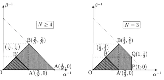
asFigure 2: Admissible exponents for (K2) and (K3)
Now it is possible to take $k(x, y)=W(x-y)$ in the definition ofintegral operator
(4.1)
as
in the usual Hartree equations. In this context let $W\in L_{1oc}^{1}(\mathbb{R}^{N})$ satisfy thefollowingthree conditions:
(Wl) $W$ is
a
real-valuedeven
function, that is, $W(-x)=W(x)\in \mathbb{R}$a.a.
$x\in \mathbb{R}^{N}$;(W2) There exists$p \geq\max\{1, N/4\}$ such that $W\in L^{\infty}(\mathbb{R}^{N})+L^{p}(\mathbb{R}^{N})$;
$(W3\rangle$ There exists $q \geq N/2 such that W_{-};=-\min\{W, 0\}\in L^{\infty}(\mathbb{R}^{N})+L^{q}(\mathbb{R}^{N})$
.
We can show that $k(x, y)=W(x-y)$ belongs to $L_{x}^{\infty}(L_{y}^{\infty})+L_{x}^{\infty}(L_{y}^{1\vee(N/4\rangle})$
.
Thus theadmissiblepair intheconvolutioncaseislocatedonthe edge$OA(N\geq 4)$or $OP(N=3)$
as
in Figure 2. Hencewe
have thefollowing:Corollary 4.2. Let$N\geq 3$ and$a>-(N-2)^{2}/4$, Assume that$W$
satisfies
$(W1)-(W3)$.
Then
for
every$u_{0}\in H^{1}(\mathbb{R}^{N})$ there $ex’ists$ a unique global weak solution$u$ to(4.5) $i \frac{\partial u}{\theta t}=-\Delta u+\frac{a}{|x|^{2}}u+(W*|u|^{2})u$ in$\mathbb{R}\cross \mathbb{R}^{N},$
$u(O, x)=u_{0}(x)$ in$\mathbb{R}^{N}.$
Moreover, $u$
satisfies
conservation laws (4.4) with(4.6) $E( \varphi):=\frac{1}{2}\Vert\nabla\varphi\Vert_{L^{2}}^{2}+\frac{a}{2}\Vert\frac{\varphi}{|x|}\Vert_{L^{2}}^{2}$
$+ \frac{1}{4}\int_{\mathbb{R}^{N}}\int_{\mathbb{R}^{N}}W(x-y)|\varphi(x)|^{2}|\varphi(y)|^{2}dxdy, \varphi\in H^{1}(\mathbb{R}^{N})$
.
Proofof Corollary 4.2. By virtue of Theorem 4.1, it suffices to show that $k(x, y);=$
and (K3), that is, $k$ belongs to $L_{x}^{\infty}(L_{y}^{\infty})+L_{x}^{\infty}(L_{y}^{1\vee(N/4)})$ and $k_{-}$ belongs to $L_{x}^{\infty}(L_{y}^{\infty})+$ $L_{x}^{\infty}(L_{y}^{N/2})$
.
For $R>0$ set$W_{R}(x):=\{\begin{array}{l}W(x) (|W(x)|\leq R) ,R (W(x)>R) ,-R (W(x)<-R) .\end{array}$
Then we have $|W_{R}(x)|\leq R$
on
$\mathbb{R}^{N}$so
that(4.7) $|W(x)|\leq|W(x)-W_{R}(x)|+|W_{R}(x)|\leq|W(x)-W_{R}(x)|+R.$
By (W2) we have $W-W_{R}\in L^{q(N)}(\mathbb{R}^{N})$, where $q(N):=(N/4)\vee 1$
.
Hence$\int_{\mathbb{R}^{N}}|W(x-y)-W_{R}(x-y)|^{q(N)}dx=\int_{\mathbb{R}^{N}}|W(x)-W_{R}(x)|^{q(N)}dx$
$=\Vert W-W_{R}\Vert_{L^{q(N)}}^{q(N)} \forall y\in \mathbb{R}^{N}.$
Thus we obtain
$\Vert k-k_{R}\Vert_{L_{x}(L_{y}^{q(N)})}\infty=\Vert W-W_{R}\Vert_{L^{q(N)}}arrow 0 (Rarrow\infty)$
.
Therefore $k(x, y)=W(x-y)$ belongs to $L_{x}^{\infty}(L_{y}^{\infty})+L_{x}^{\infty}(L_{y}^{q(N)})$ andsatisfies (K2).
Since $k_{-}(x, y)=W_{-}(x-y)$, we conclude that $k_{-}$ belongs to $L_{x}^{\infty}(L_{y}^{\infty})+L_{x}^{\infty}(L_{y}^{N/2})$
and satisfies (K3) in a way similar to (K2). $I$
5. Proof of
Theorem
4.1
In [13] the proofof Theorem 4.1 is mostly omitted. Thus we fully give the proof of
Theorem 4.1 in this section. Toshow Theorem 4.1 weverify (Gl)$-(G6)$ with
(5.1) $g(u)(x):=(uK(|u|^{2}))(x)=u(x) \int_{\mathbb{R}^{N}}k(x, y)|u(y)|^{2}dy, u\in H^{1}(\mathbb{R}^{N})$,
(5.2) $G(u):= \frac{1}{4}\int_{\mathbb{R}^{N}}\int_{\mathbb{R}^{N}}k(x, y)|u(x)|^{2}|u(y)|^{2}dxdy, u\in H^{1}(\mathbb{R}^{N})$
and the uniqueness of local weaksolutions to $(HE)_{a}.$
First we show the uniqueness of local weak solutions to $(HE)_{a}$
.
To prove it, weuse the Strichartz estimates for $\{e^{-itP_{a}}\}$ established by Burq, Planchon, Stalker and
Tahvildar-Zadeh[1] (see also [10, Theorems 2.3 and 2.5]):
Lemma 5.1. Let $N\geq 3$ and $(p, q)$ be a Schr\"odinger admissible pair, i. e.,
Then the following inequality holds:
(5.3) $\Vert e^{-itP_{a}}\varphi\Vert_{Lp(\mathbb{R};L^{q})}\leq C\Vert\varphi\Vert_{L^{2}} \forall\varphi\in L^{2}(\mathbb{R}^{N})$
.
Moreover let $(p_{j}, q_{j})(j=1,2)$ be Schr\"odinger admissible pairs. Then
(5.4) $\Vert\int_{0}^{t}e^{-i(t-s)P_{a}}\Phi(s, x)d_{\mathcal{S}}\Vert_{L^{p_{2}}(\mathbb{R};L^{q_{2}})}\leq C’\Vert\Phi\Vert_{L^{p_{1}’}(\mathbb{R};L^{q_{1}’})}$ $\forall\Phi\in L^{p_{1}’}(\mathbb{R};L^{q_{1}’}(\mathbb{R}^{N}))$.
In fact the endpoint case$p_{1}=2=p_{2}$ in (5.4) has been restricted in [10, Theorems
2.5]. But we can
remove
the restriction by Pierfelice[12, Theorem 2 in Section 3] (seealso [2, Theorem 3]$)$.
Lemma 5.2. Let$u_{j}(j=1,2)$ be local weak solutions to $(HE)_{a}$ on $(-T, T)$ with initial
values$u_{j}(0)=u_{j,0}$
.
Thenfor
$t\in(-T, T)$(5.5) $\Vert u_{1}(t)-u_{2}(t)\Vert_{L^{2}}\leq C\Vert u_{1,0}-u_{2,0}\Vert_{L^{2}},$
where $C$ is a constant depending on $\Vert u_{j}\Vert_{L(-T,T;L^{2})}\infty$ and $\Vert u_{j}\Vert_{L^{\infty}(-T,T;L^{2\gamma})}(j=1,2)$. Proof. Let $u_{j}\in L^{\infty}(I;H^{1}(\mathbb{R}^{N}))(j=1,2)$ belocal weaksolutions to $(HE)_{a}$ on$(-T, T)$
with initial values $u_{j}(0)=u_{j,0}$
.
Then $u_{j}(j=1,2)$ satisfy the following integralequa-tions:
$u_{j}(t)=e^{-itP_{a}}u_{j,0}-i \int_{0}^{t}e^{-i(t-s)P_{a}}g(u_{j}(s))ds.$
Therefore we
see
that $v(t)$ $:=u_{1}(t)-u_{2}(t)$ satisfies$v(t)=e^{-itP_{a}}[u_{1,0}-u_{2,0}]-i \int_{0}^{t}e^{-i(t-s)P_{a}}[g(u_{1}(s))-g(u_{2}(s))]d_{\mathcal{S}}.$
Now let $(r(\gamma), 2\gamma)$ be a Schr\"odinger admissible pair:
$\frac{2}{r(\gamma)}+\frac{N}{2\gamma}=\frac{N}{2}$, i.e., $r( \gamma):=\frac{4\gamma}{N(\gamma-1)}.$
Applying (5.23), (5.24) and the Strichartz estimates (5.3), (5.4), we see that for every
Schr\"odinger admissible pair $(\tau, \rho)$,
(5.6) $\Vert e^{-itP_{a}}[u_{1,0}-u_{2,0}]\Vert_{L^{\tau}(-T,T;L\rho})\leq C_{\tau}\Vert u_{1,0}-u_{2,0}\Vert_{L^{2}},$ (5.7) $\Vert\int_{0}^{t}e^{-i(t-s)P_{a}}[g_{1}(u_{1}(\mathcal{S}))-g_{1}(u_{2}(s))]ds\Vert_{L^{\tau}(-T,T;L\rho)}$
$\leq C_{\infty,\tau}\Vert g_{1}(u_{1})-g_{1}(u_{2})\Vert_{L^{1}(-T,T;L^{2})}$
$\leq 2C_{\infty,\tau}RT[\Vert u_{1}\Vert_{L_{t}^{\infty}L^{2}}^{2}+\Vert u_{1}\Vert_{L_{t}^{\infty}L^{2}}\Vert u_{2}\Vert_{L_{t}^{\infty}L^{2}}+\Vert u_{2}\Vert_{L_{t}^{\infty}L^{2}}^{2}]\Vert v\Vert_{L(-T,T;L^{2})}\infty,$
(5.8) $\Vert\int_{0}^{t}e^{-i(t-s)P_{a}}[g_{2}(u_{1}(s))-g_{2}(u_{2}(s))]ds\Vert_{L^{\tau}(-T,T;L^{\rho})}$
$\leq C_{r(\gamma),\tau}\Vert g_{2}(u_{1})-g_{2}(u_{2})\Vert_{L^{r(\gamma)’}()}-\tau,\tau_{;L(2\gamma)’}$
$\leq C_{r(\gamma),\tau}(2T)^{1-2/r(\gamma)}\Vert\ell_{R}\Vert_{\mathcal{B}(\alpha,\beta)}$
where $\Vert\cdot\Vert_{L_{t}^{\infty}L^{p}}$ $:=\Vert\cdot\Vert_{L}\infty(-T,T;L^{p})$
.
Putting $(\tau, \rho)$ $:=(\infty, 2)$ and $(\tau, \rho)$ $:=(r(\gamma), 2\gamma)$ in (5.6), (5.7) and (5.8),
we see
that(5.9) $\Vert v\Vert_{L^{r(\gamma)}(-T,T;L^{2\gamma})}+\Vert v\Vert_{L^{\infty}(-T,T;L^{2})}$
$\leq(C_{r(\gamma)}+C_{\infty})\Vert u_{1,0}-u_{2,0}\Vert_{L^{2}}+6(C_{\infty,\infty}+C_{\infty,r(\gamma)})RM^{2}T\Vert v\Vert_{L^{\infty}(-T,T;L^{2})}$
$+3(C_{r(\gamma),\infty}+C_{r(\gamma),r(\gamma)})\Vert\ell_{R}\Vert_{L_{x}^{\beta}(L_{y}^{\alpha})}M^{2}(2T)^{1-2/r(\gamma)}\Vert v\Vert_{L^{r(\gamma)}(-T,T;L^{2\gamma})},$
where
$M:=_{j} \max_{=1,2}\{\Vert u_{j}\Vert_{L^{\infty}(-T,T;L^{2})}\vee\Vert u_{j}\Vert_{L}\infty(-\tau,\tau;L^{2\gamma})\}.$
Case 1 $(\alpha^{-1}+\beta^{-1}<4/N)$
.
Take$T_{0}\in(0, T)$ such that $6(C_{\infty,\infty}+C_{\infty,r(\gamma)})RM^{2}T_{0}\leq 1/2$and $3(C_{r(\gamma),\infty}+C_{r(\gamma),r(\gamma)})\Vert\ell_{R}\Vert_{L_{x}^{\beta}(L_{y}^{\alpha})}M^{2}(2T_{0})^{1-2/r(\gamma)}\leq 1/2$
.
Then by (5.9) we obtain(5.10) $\Vert v\Vert_{L^{r(\gamma)}(-T_{0},T_{0};L^{2\gamma})}+\Vert v\Vert_{L^{\infty}(-T_{0},T_{0};L^{2})}\leq 2(C_{r(\gamma)}+C_{\infty})\Vert u_{1,0}-u_{2,0}\Vert_{L^{2}}.$
Case 2 $(\alpha^{-1}+\beta^{-1}=4/N)$
.
This is thecriticalcase
because of$2\gamma=2N/(N-2)$.
Thenwe
see
from (5.9) that$\Vert v\Vert_{L^{2}()}-\tau,\tau_{;L^{2N/(N-2)}}+\Vert v\Vert_{L}\infty(-T,T;L^{2})$
$\leq(C_{2}+C_{\infty})\Vert u_{1,0}-u_{2,0}\Vert_{L^{2}}+6(C_{\infty,\infty}+C_{\infty,2})RM^{2}T\Vert v\Vert_{L(-T,T;L^{2})}\infty$
$+3(C_{2,\infty}+C_{2,2})\Vert\ell_{R}\Vert_{L_{x}^{\beta}(L_{y}^{\alpha})}M^{2}\Vert v\Vert_{L^{2}(-T,T;L^{2N/(N-2))}}.$
Fix $R>0$ so that $3(C_{2,\infty}+C_{2,2})\Vert\ell_{R}\Vert_{L_{x}^{\beta}(L_{y}^{\alpha})}M^{2}\leq 1/2$
.
Next take $T_{0}\in(0, T)$ such that $6(C_{\infty,\infty}+C_{\infty,r(\gamma)})RM^{2}T_{0}\leq 1/2$.
Then wehave (5.10).Extendingthe interval step by step, weconclude (5.5). $I$
Selecting$u_{0,1}=u_{0,2}$, we
see
that $u_{1}=u_{2}$ in$L^{\infty}(-T, T;H^{1}(\mathbb{R}^{N}))$.
Hencewe
concludethe uniqueness oflocal weak solutions to $(HE)_{a}$
on
$(-T, T)$.
Next we verify (Gl)$-(G6)$. To end this, we applythe following two lemmas.
Lemma 5.3 ([13, Lemma 2.4]). Let $\alpha,$ $\beta,$ $\gamma,$ $\rho\in[1, \infty]$
.
Assume that $k\in L_{x}^{\beta}(L_{y}^{\alpha})\cap$$L_{y}^{\beta}(L_{x}^{\alpha})$ and
$\alpha\leq\rho\leq\beta, \frac{1}{\alpha}+\frac{1}{\beta}+\frac{1}{\gamma}=1+\frac{1}{\rho}.$
Then the opemtor
defined
by (4.1) is linear and boundedfrom
$L^{\gamma}(\mathbb{R}^{N})$ to$L^{\rho}(\mathbb{R}^{N})$.
More-over
(5.11) $\Vert Kf\Vert_{L\rho(\mathbb{R}^{N})}\leq(\Vert k\Vert_{L_{x}^{\beta}(L_{y}^{\alpha})}\vee\Vert k\Vert_{L_{y}^{\beta}(L_{x}^{\alpha})})\Vert f\Vert_{L^{\gamma}(\mathbb{R}^{N})} \forall f\in L^{\gamma}(\mathbb{R}^{N})$
.
Lemma 5.4 ([13, Lemma 2.5]). Let$\alpha,$ $\beta\in[1, \infty]$ be two exponents such that$\alpha\leq\beta$ and $\alpha^{-1}+\beta^{-1}\leq 4/N$
.
Put$\gamma^{-1}$ $:=1-(\alpha^{-1}+\beta^{-1})/2$. Assume that$k\in L_{x}^{\beta}(L_{y}^{\alpha})$ is symmetric.Then
for
all$u_{j}\in H^{1}(\mathbb{R}^{N})(j=1,2,3,4)$(5.12) $\Vert u_{1}K(u_{2}\overline{u}_{3})\Vert_{L(2\gamma)’}\leq\Vert k\Vert_{L_{x}^{\beta}(L_{y}^{\alpha})}\Vert u_{1}\Vert_{L^{2\gamma}}\Vert u_{2}\Vert_{L^{2\gamma}}\Vert u_{3}\Vert_{L^{2\gamma}},$
Now we start to verify (Gl)$-(G6)$
.
Verification of (Gl). Let $u,$ $v\in H^{1}(\mathbb{R}^{N})$
.
Then we see from (Kl) that(5.14) $G(u+v)-G(u)-{\rm Re}\langle g(u), v\rangle_{H^{-1},H^{1}}$
$= \frac{1}{4}\int_{\mathbb{R}^{N}}\int_{\mathbb{R}^{N}}k(x, y)[|(u+v)(x)|^{2}|(u+v)(y)|^{2}-|u(x)|^{2}|u(y)|^{2}]dxdy$
- $\frac{1}{4}\int_{\mathbb{R}^{N}}\int_{\mathbb{R}^{N}}k(x, y)[2{\rm Re}(u(x)\overline{v}(x))|u(y)|^{2}+2{\rm Re}(u(y)\overline{v}(y))|u(x)|^{2}]dxdy.$
Now let $A,$ $B,$ $\xi,$ $\eta\in \mathbb{C}$
.
Thenwe see
that(5.15) $|A+\xi|^{2}|B+\eta|^{2}-|A|^{2}|B|^{2}-2|B|^{2}{\rm Re}(A\overline{\xi})-2|A|^{2}{\rm Re}(B\overline{\eta})$
$=4{\rm Re}(A\overline{\xi}){\rm Re}(B\overline{\eta})+|\xi|^{2}(|B|^{2}+2{\rm Re}(B\overline{\eta}))+|\eta|^{2}(|A|^{2}+2{\rm Re}(A\overline{\xi}))+|\xi|^{2}|\eta|^{2}$
Put $A:=u(x),$ $B:=u(y),$ $\xi=v(x),$ $\eta=v(y)$ in (5.15). It follows from (5.14) that
(5.16) $G(u+v)-G(u)-{\rm Re}\langle g(u), v\rangle_{H^{-1},H^{1}}=I_{1}+I_{2}+I_{3},$
where
$I_{1}:= \int_{\mathbb{R}^{N}}\int_{\mathbb{R}^{N}}k(x, y){\rm Re}(u(x)\overline{v}(x)){\rm Re}(u(y)\overline{v}(y))dxdy,$
$I_{2}:= \frac{1}{2}\int_{\mathbb{R}^{N}}\int_{\mathbb{N}^{N}}k(x, y)|v(x)|^{2}(|u(y)|^{2}+2{\rm Re}(u(y)\overline{v}(y)))dxdy,$
$I_{3}:= \frac{1}{4}\int_{\mathbb{R}^{N}}\int_{\mathbb{R}^{N}}k(x, y)|v(x)|^{2}|v(y)|^{2}dxdy.$
Now let $R>0$ so that $\ell_{R}\in L_{x}^{\beta}(L_{y}^{\alpha})$
.
First we see for $I_{1}$ that$|I_{1}| \leq\int_{\mathbb{R}^{N}}\int_{\mathbb{R}^{N}}|k_{R}(x, y)||u(x)||v(x)||u(y)||v(y)|dxdy$
$+ \int_{\mathbb{R}^{N}}\int_{\mathbb{R}^{N}}|\ell_{R}(x, y)||u(x)||v(x)||u(y)||v(y)|dxdy.$
Applying Lemma 5.4, wehave
(5.17) $|I_{1}|\leq R\Vert u\Vert_{L^{2}}^{2}\Vert v\Vert_{L^{2}}^{2}+\Vert\ell_{R}\Vert_{L_{x}^{\beta}(L_{y}^{\alpha})}\Vert u\Vert_{L^{2\gamma}}^{2}\Vert v\Vert_{L^{2\gamma}}^{2}.$ $\leq R\Vert u\Vert_{H^{1}}^{2}\Vert v\Vert_{H^{1}}^{2}+c^{4}\Vert\ell_{R}\Vert_{L_{x}^{\beta}(L_{y}^{\alpha})}\Vert u\Vert_{H^{1}}^{2}\Vert v\Vert_{H^{1}}^{2}.$ In asimilar way of theestimates for $I_{1}$, we see that
(518) $|I_{2}|\leq\dashv_{2}^{R}|v\Vert_{H^{1}}^{2}(\Vert u\Vert_{H^{1}}^{2}+2\Vert u\Vert_{H^{1}}\Vert v\Vert_{H^{1}})$
$+ \frac{c^{4}}{2}\Vert l_{R}\Vert_{L_{x}^{\beta}(L_{y}^{\alpha})}\Vert v\Vert_{H^{1}}^{2}(\Vert u\Vert_{H^{1}}^{2}+2\Vert u\Vert_{H^{1}}\Vert v\Vert_{H^{1}})$
,
Since $L^{2\gamma}(\mathbb{R}^{N})\subset H^{1}(\mathbb{R}^{N})$
we
have from (5.16), (5.17), (5.18) and (5.19) that(5.20) $|G(u+v)-G(u)-{\rm Re}\langle g(u), v\rangle_{H^{-1},H^{1}}|$
$\leq\frac{R+c^{4}\Vert\ell_{R}\Vert_{L_{x}^{\beta}(L_{y}^{\alpha})}}{4}\Vert v\Vert_{H^{1}}^{2}(6\Vert u\Vert_{H^{1}}^{2}+4\Vert u\Vert_{H^{1}}\Vert v\Vert_{H^{1}}+\Vert v\Vert_{H^{1}}^{2})$
.
Let $M>0$ and$\epsilon>0$
.
Then wesee
that$|G(u+v)-G(u)-{\rm Re}\langle g(u),$$v \rangle_{H^{-1},H^{1}}|\leq\frac{R+c^{4}\Vert\ell_{R}\Vert_{L_{x}^{\beta}(L_{y}^{\alpha})}}{4}(6M^{2}+4M+1)\Vert v\Vert_{H^{1}}^{2}$
$\forall u,$ $v\in H^{1}(\mathbb{R}^{N})$ with $\Vert u\Vert_{H^{1}}\leq M,$ $\Vert v\Vert_{H^{1}}\leq 1.$
Hence by setting $\delta>0$ as
$\delta=\delta(u,\epsilon)=1\wedge\frac{4\epsilon}{(R+c^{4}\Vert\ell_{R}\Vert_{L_{x}^{\beta}(L_{y}^{\alpha})})(6M^{2}+4M+1)},$
we conclude that
$|G(u+v)-G(u)-{\rm Re}\langle g(u),$$v\rangle_{H^{-1},H^{1}}|\leq\epsilon\Vert v\Vert_{H^{1}}$ $\forall v\in H^{1}(\mathbb{R}^{N})$ with $\Vert v\Vert_{H^{1}}\leq\delta.$
This is nothing but (Gl).
Verification of (G2). Let $u,$ $v\in H^{1}(\mathbb{R}^{N})$. Then
we
see
that$g(u)-g(v)=K(|u|^{2})u-K(|v|^{2})v=K(|u|^{2}-|v|^{2})u+K(|v|^{2})(u-v)$
.
Now we divide $K$ into $K_{R}$ and $L_{R}$ as
(5.21) $K_{R}(f)(x) := \int_{\mathbb{R}^{N}}k_{R}(x, y)f(y)dy,$
(5.22) $L_{R}(f)(x) := \int_{R^{N}}\ell_{R}(x, y)f(y)dy.$
Note that $K=K_{R}+L_{R}$. Applying 5.4 with $L_{x}^{\infty}(L_{y}^{\infty})$ and $\Vert k_{R}\Vert_{L_{x}(L_{y}^{\infty})}\infty\leq R$ we have
(5.23) $\Vert K_{R}(|u|^{2})u-K_{R}(|v|^{2})v\Vert_{H^{-1}}$
$\leq\Vert K_{R}(|u|^{2}-|v|^{2})u\Vert_{L^{2}}+\Vert K_{R}(|v|^{2})(u-v)\Vert_{L^{2}}$
$\leq R(\Vert u\Vert_{L^{2}}+\Vert v\Vert_{L^{2}})\Vert u-v\Vert_{L^{2}}\Vert u\Vert_{L^{2}}+R\Vert v\Vert_{L^{2}}^{2}\Vert u-v\Vert_{L^{2}}$
$\leq R(\Vert u\Vert_{L^{2}}^{2}+\Vert u\Vert_{L^{2}}\Vert v\Vert_{L^{2}}+\Vert v\Vert_{L^{2}}^{2})\Vert u-v\Vert_{L^{2}}.$
On the other hand, applying Lemma 5.4 with $L_{x}^{\beta}(L_{y}^{\alpha})$ we have (5.24) $c^{-1}\Vert L_{R}(|u|^{2})u-L_{R}(|v|^{2})v\Vert_{H}-1$
$\leq\Vert L_{R}(|u|^{2})u-L_{R}(|v|^{2})v\Vert_{L(2\gamma)’}$
$\leq\Vert\ell_{R}\Vert_{L_{x}^{\beta}(L_{y}^{\alpha})}(\Vert u\Vert_{L^{2\gamma}}^{2}+\Vert u\Vert_{L^{2\gamma}}\Vert v\Vert_{L^{2\gamma}}+\Vert v\Vert_{L^{2\gamma}}^{2})\Vert u-v\Vert_{L^{2\gamma}}$
Combining (5.23) and (5.24), we obtain (G2):
(5.25) $\Vert g(u)-g(v)\Vert_{H}-1\leq R(\Vert u\Vert_{L^{2}}^{2}+\Vert u\Vert_{L^{2}}\Vert v\Vert_{L^{2}}+\Vert v\Vert_{L^{2}}^{2})\Vert u-v\Vert_{L^{2}}.$
$+c^{4}\Vert\ell_{R}\Vert_{L_{x}^{\beta}(L_{y}^{\alpha})}(\Vert u\Vert_{H^{1}}^{2}+\Vert u\Vert_{H^{1}}\Vert v\Vert_{H^{1}}+\Vert v\Vert_{H^{1}}^{2})\Vert u-v\Vert_{H^{1}}$
$\leq 3M^{2}(R+c^{4}\Vert\ell_{R}\Vert_{L_{x}^{\beta}(L_{y}^{\alpha})})\Vert u-v\Vert_{H^{1}}$
$\forall u,$ $v\in H^{1}(\mathbb{R}^{N})$ with $\Vert u\Vert_{H^{1}},$ $\Vert v\Vert_{H^{1}}\leq M.$
Verification of (G3). Let $u,$ $v\in H^{1}(\mathbb{R}^{N})$ with $\Vert u\Vert_{H^{1}},$ $\Vert v\Vert_{H^{1}}\leq M$. Then we see from
(Kl) that
$G(u)-G(v)= \frac{1}{4}\int_{\mathbb{R}^{N}}\int_{\mathbb{R}^{N}}k(x, y)(|u(y)|^{2}-|v(y)|^{2})(|u(x)|^{2}+|v(x)|^{2})dxdy.$
Thus we evaluate the following two integrals:
$I(k_{R}) := \frac{1}{4}\int_{\mathbb{R}^{N}}\int_{\mathbb{R}^{N}}k_{R}(x, y)(|u(y)|^{2}-|v(y)|^{2})(|u(x)|^{2}+|v(x)|^{2})dxdy,$
$I( \ell_{R}) :=\frac{1}{4}\int_{\mathbb{R}^{N}}\int_{\mathbb{N}^{N}}\ell_{R}(x,y)(|u(y)|^{2}-|v(y)|^{2})(|u(x)|^{2}+|v(x)|^{2})dxdy.$
Note that $G(u)-G(v)=I(k_{R})+I(\ell_{R})$. For $I(k_{R})$ we calculate
$|I(k_{R})| \leq\frac{R}{4}\Vert u-v\Vert_{L^{2}}(\Vert u\Vert_{L^{2}}+\Vert v\Vert_{L^{2}})(\Vert u\Vert_{L^{2}}^{2}+\Vert v\Vert_{L^{2}}^{2})\leq RM^{3}\Vert u-v\Vert_{L^{2}}.$
On the other hand, for $I(\ell_{R})$ we evaluate
$|I( \ell_{R})|\leq\frac{\Vert\ell_{R}\Vert_{L_{x}^{\beta}(L_{y}^{\alpha})}}{4}(\Vert u\Vert_{L^{2\gamma}}^{2}+\Vert v\Vert_{L^{2\gamma}}^{2})^{2}\leq c^{4}\Vert\ell_{R}\Vert_{L_{x}^{\beta}(L_{y}^{\alpha})}M^{4}.$
By virtue of (K2), we see that
(5.26) $\Vert\ell_{R}\Vert_{L_{x}^{\beta}(L_{y}^{\alpha})}=\Vert k-k_{R}\Vert_{L_{x}^{\beta}(L_{y}^{\alpha})}arrow 0$ as $Rarrow\infty.$
Hence for every $\delta>0$ there exists $R(\delta)>0$ such that
$\Vert\ell_{R(\delta)}\Vert_{L_{x}^{\beta}(L_{y}^{a})} c^{4}M^{4}.$
$<\underline{\delta}$
Thus for all $u,$ $v\in H^{1}(\mathbb{R}^{N})$ with $\Vert u\Vert_{H^{1}},$ $\Vert v\Vert_{H^{1}}\leq M$ we have
$|G(u)-G(v)|\leq\delta+R(\delta)M^{3}\Vert u-v\Vert_{L^{2}} \forall\delta>0.$
This is nothing but (G3).
Verification of (G4). Let $u\in H^{1}(\mathbb{R}^{N})$
.
Then (Kl) implies (G4):Verification of (G5). Let $\{w_{n}\}_{n}$ be
a
sequence in $L^{\infty}(I;H^{1}(\mathbb{R}^{N}))$ satisfying(5.27) $\{\begin{array}{ll}w_{n}(t)arrow w(t)(narrow\infty) weakly in H^{1}(\mathbb{R}^{N}) a.a.t\in I,g(w_{n})arrow f(narrow\infty) weakly^{*} in L^{\infty}(I;H^{-1}(\mathbb{R}^{N})) .\end{array}$
Define $\sigma_{1}$ $:=2,$ $\sigma_{2}$ $:=2\gamma$ and
$g_{1}(u):=u(x) \int_{\mathbb{R}^{N}}k_{R}(x, y)|u(y)|^{2}dy, g_{2}(u):=u(x)\int_{\mathbb{R}^{N}}\ell_{R}(x, y)|u(y)|^{2}dy.$
Since $\{g_{1}(w_{n})\}_{n}$ and $\{g_{2}(w_{n})\}_{n}$arebounded in $L^{\infty}(I;H^{-1}(\mathbb{R}^{N}))$ and theSobolev
embed-dings, there exist a subsequence $\{w_{n(j)}\}_{j}$ of $\{w_{n}\}_{n}$ and $f_{1},$ $f_{2}\in L^{\infty}(I;H^{-1}(\mathbb{R}^{N}))$ such
that
(5.28) $g_{l}(w_{n(j)})arrow f_{l}(jarrow\infty)$ $weakly^{*}$ in$L^{\infty}(I;L^{\sigma_{l}’}(\mathbb{R}^{N}))(l=1,2)$
.
To confirrn (2.2) let $fl\subset \mathbb{R}^{N}$ be an arbitrary bounded open subset with $C^{1}$ boundary.
Then
(5.29) $\langle f|(t), w(t)\rangle_{L^{\sigma_{l}’}(\zeta\}),L^{\sigma}t(\zeta\})}=\langle f_{l}(t)-g_{l}(w_{n(j)}(t)), w(t)\rangle_{L^{\sigma_{l}’}(\zeta\}),L^{\sigma_{l}}(\zeta\})}$
$+\langle g_{l}(w_{n(j)}(t)), w(t)-w_{n(j)}(t)\rangle_{L^{\sigma_{l}’}(\downarrow 1),L^{\sigma_{l}}(ll)}$
$+\langle g_{l}(w_{n(j)}(t)), w_{n(j)}(t)\rangle_{L^{\sigma_{l}’}(l),L^{\sigma_{l}}(\iota\iota)}$
$=:I_{l1}(t)+I_{l2}(t)+I_{l3}(t) (l=1,2)$
.
The weak convergence (5.28) asserts that
(5.30) $lI_{l1}(t)dtarrow 0(jarrow\infty) , l=1,2.$
Next we consider $I_{l2}(l=1,2)$
.
Rellich’s compactness theorem implies that $w_{n(j)}(t)arrow$$w(t)(jarrow\infty)$ strongly in $L^{2}(\zeta l)$ a.a. $t\in I$
.
Hence it follows from the boundedness of$\{g_{1}(w_{n(j)}(t))\}_{j}$ in $L^{2}(\zeta l)$ a.a. $t\in I$that $I_{12}(t)arrow 0(jarrow\infty)$ for a.a. $t\in I$
.
Moreover, the boundedness of $\{w_{n(j)}\}_{j}$ and $\{g_{1}(w_{n(j)})\}_{j}$ in $L^{\infty}(I;L^{2}(fl))$ implies that(5.31) $lI_{12}(t)dtarrow 0(jarrow\infty)$.
On the other hand, for $I_{22}$ we evaluate $|I_{22}(t)|\leq 2M^{4}c^{4}\Vert\ell_{R}\Vert_{L_{x}^{\beta}(L_{y}^{\alpha})}$
.
Note that theconstant 2$M^{4}c^{4}\Vert\ell_{R}\Vert_{L_{x}^{\beta}(L_{y}^{\alpha})}$ does not depend on $\zeta l_{d’X1}dj$
.
Hencewe haveSince and arereal-valued, weseethat${\rm Im} I_{\iota 3}(t)=0$ a.a. $t\in I(l=1,2)$
.
Integrating (5.29) over $I$ and using (5.30), (5.31) and (5.32), we obtain${\rm Im} \int_{I}\langle f_{1}(t), w(t)\rangle_{L^{2}(\zeta\})}dt=0,$
$|{\rm Im} l\langle f_{2}(t), w(t)\rangle_{L(t\}),L^{2\gamma}(t1)}(2\gamma)’dt|\leq 2|I|M^{4}c^{4}\Vert P_{R}\Vert_{L_{x}^{\beta}(L_{y}^{\alpha})}.$
Since S2 is arbitrary $A^{r}1df=f_{1}+f_{2}$,
we
obtain (2.2) by letting $Rarrow\infty$ and using (G4):${\rm Im} l \langle f(t), w(t)\rangle_{H^{-1},H^{1}}dt=0=\lim_{narrow\infty}{\rmIm} l\langle g(w_{n}(t)), w_{n}(t)\rangle_{H^{-1},H^{1}}dt.$
Next we show that $f=g(w)$ by assuming further that $w_{n}(t)arrow w(t)(narrow\infty)$ in
$L^{2}(\mathbb{R}^{N})$ a.a. $t\in I$
.
Let $M:= \sup_{n}\Vert w_{n}\Vert_{L\infty(I;H^{1})}$. It follows from (5.25) that $\Vert g(w_{n}(t))-g(w(t))\Vert_{H^{-1}}\leq 3M^{2}R\Vert w_{n}(t)-w(t)\Vert_{L^{2}}+6c^{4}M^{4}\Vert\ell_{R}\Vert_{L_{x}^{\beta}(L_{y}^{\alpha})}.$Passing to the limit as $narrow\infty$, we obtain
$\lim_{narrow}\sup_{\infty}\Vert g(w_{n}(t))-g(w(t))\Vert_{H^{-1}}\leq 6c^{4}M^{4}\Vert\ell_{R}\Vert_{L_{x}^{\beta}(L_{y}^{\alpha})}$ a.a. $t\in I.$
Since $R$ is arbitrary, we see that $g(w_{n}(t))arrow g(w(t))(narrow\infty)$ in $H^{-1}(\mathbb{R}^{N})$ a.a. $t\in I.$
Therefore we conclude that $f=g(w)$ and (G5) is verified.
Verification of (G6). Let $k_{-}(x, y);=(-k(x, y))\vee O$ and
(5.33) $k_{R}^{-}(x, y)$ $:=\{\begin{array}{ll}k_{-}(x, y) k^{-}(x, y)\leq R,R k^{-}(x, y)>R,\end{array}$
(5.34) $\ell_{R}^{-}(x, y):=k_{-}(x, y)-k_{R}^{-}(x, y)$.
Then we see from (5.2) and (K3) that
$G(u) \geq-\frac{1}{4}\int_{\mathbb{R}^{N}}\int_{\mathbb{R}^{N}}k_{R}^{-}(x, y)|u(x)|^{2}|u(y)|^{2}dxdy$
$- \frac{1}{4}\int_{\mathbb{R}^{N}}\int_{\mathbb{R}^{N}}\ell_{R}^{-}(x, y)|u(x)|^{2}|u(y)|^{2}dxdy \forall u\in H^{1}(\mathbb{R}^{N})$
.
Applying Lemma 5.4, we have for $u\in H^{1}(\mathbb{R}^{N})$,
$- \frac{1}{4}\int_{\mathbb{R}^{N}}\int_{\mathbb{R}^{N}}k_{R}^{-}(x, y)|u(x)|^{2}|u(y)|^{2}dxdy\geq-\frac{1}{4}R\Vert u\Vert_{L^{2}}^{4},$
where $\tilde{\gamma}^{-i}=1-(\tilde{\alpha}^{-1}+\tilde{\beta}^{-1})/2$
.
It follows from theGagliardo-Nirenberg inequality that(5.35) $\Vert u\Vert_{L^{2\tilde{\gamma}}}\leq c_{0}\Vert u\Vert_{L^{2}}^{1-\theta}||\nabla u\Vert_{L^{2}}^{\theta} \forall u\in H^{1}(\mathbb{R}^{N})$ ,
where
$\theta=N(\frac{1}{2}-\frac{1}{2\gamma})=\frac{N}{4}(\frac{1}{\tilde{\alpha}}+\frac{1}{\tilde{\beta}})$
.
Case 1 $(\tilde{\alpha}^{-1}+\tilde{\beta}^{-1}<2/N)$
.
Note that $N(\tilde{\alpha}^{-1}+\tilde{\beta}^{-1})<2$.
Hence (5.35) andthe Younginequality imply that
$- \frac{1}{4}\Vert\ell_{R}^{-}\Vert_{L_{x}^{\overline{\beta}}(L_{y}^{\tilde{\alpha}})}\Vert u\Vert_{L^{2\overline{\gamma}}}^{4}\geq-c_{0}^{4}\Vert\ell_{R}^{-}\Vert_{L_{x}^{\overline{\beta}}(L_{y}^{\overline{\alpha}})}\Vert u\Vert_{L^{2}}^{4-N(\tilde{\alpha}^{-1}+\tilde{\beta}^{-1})}\Vert\nabla u\Vert_{L^{2}}^{N(\tilde{\alpha}^{-1}+\tilde{\beta}^{-1})}$
$\geq-\delta\Vert\nabla u\Vert_{L^{2}}^{2}-C_{\delta}(\Vert u\Vert_{L^{2}}) \forall u\in H^{1}(\mathbb{R}^{N})$
.
Putting $\delta$ $:=(1-\epsilon)/2$ for some $\epsilon\in(0,1)$, we see that (G6) is satisfied.
Case 2 $(\tilde{\alpha}^{-1}+\tilde{\beta}^{-1}=2/N)$
.
This is the criticalcase.
In view of (5.35) we see that$- \frac{1}{4}\Vert\ell_{R}^{-}\Vert_{L_{x}^{\overline{\beta}}(L_{y}^{\tilde{\alpha}})}\Vert u\Vert_{L^{2\tilde{\gamma}}}^{4}\geq-c_{0}^{4}\Vert\ell_{R}^{-}\Vert_{L_{x}^{\overline{\beta}}(L_{y}^{\overline{\alpha}})}\Vert u\Vert_{L^{2}}^{2}\Vert\nabla u\Vert_{L^{2}}^{2}.$
Since $\Vert\ell_{R}^{-}\Vert_{L_{x}^{\overline{\beta}}(L_{y}^{\overline{\alpha}})}arrow 0$ as
$Rarrow\infty$ by (K3), there exists $R_{1}=R_{1}(\Vert u\Vert_{L^{2}}, \epsilon)>0$ such that
$c_{0}^{4} \Vert\ell_{R}^{-}\Vert_{L_{x}^{\tilde{\beta}}(L_{y}^{\overline{\alpha}})}\Vert u\Vert_{L^{2}}^{2}<\frac{1-\epsilon}{2}, R>R_{1}.$
Then we have
$G(u) \geq-\frac{1-\epsilon}{2}\Vert\nabla u\Vert_{L^{2}}^{2}-\frac{1}{4}R_{1}(\Vert u\Vert_{L^{2}},\epsilon)\Vert u\Vert_{L^{2}}^{4} \forall u\in H^{1}(\mathbb{R}^{N})$
.
This is nothing but (G6).
Since (Gl)$-(G6)$ areverified and the uniqueness oflocal weak solutions for $(HE)_{a}$
is proved, Theorem 2.3 yields the global existence ofweak solutions to $(HE)_{a}.$
6. Concluding remarks
Remark 6.1. In general, nonlocal nonlinearity does not satisfy the condition
(6.1) $\{\begin{array}{l}u_{n}arrow u(narrow\infty) weakly in X_{S},\Rightarrow f=g(u)g(u_{n})arrow f(narrow\infty) weakly in X_{S}^{*}\end{array}$
for any sequence $\{u_{n}\}_{n}$ in $X_{S}$ (see Section 2.3 for notations). Let $X_{S}=H^{1}(\mathbb{R}),$ $X=$
$L^{2}(\mathbb{R}),$ $X_{S}^{*}=H^{-1}(\mathbb{R})$ and consider$g(u):=\Vert u\Vert_{L^{2}}^{2}u(k(x, y)=1)$
.
Then $g$ satisfies (Gl)$-$(G6). Now we show that $g$ does not verify (6.1). Let $\varphi\in H^{1}(\mathbb{R})$ with $supp\varphi\subset[-1,1].$
Put$w_{n}(x)$ $:=\varphi(x)+\varphi(x-2n)$
.
Then $\{w_{n}\}_{n}$ is abounded sequence in $H^{1}(\mathbb{R})$.
It is easytosee that
and henceweakly in $H^{1}(\mathbb{R})$
.
Since $\Vert w_{n}\Vert_{L^{2}}^{2}=2\Vert\varphi\Vert_{L^{2}}^{2}$ for all $n\in \mathbb{N}$, we have$g(w_{n})arrow f$ $:=2\Vert\varphi\Vert_{L^{2}}^{2}\varphi$ weakly in $L^{2}(\mathbb{R})$
and hence weakly in $H^{-1}(\mathbb{R})$. But $g(\varphi)=\Vert\varphi\Vert_{L^{2}}^{2}\varphi$and so $f\neq g(\varphi)$.
Onthe other hand, local nonlinearity satisfies the condition (6.1). See [11] fordetails.
Remark 6.2. Assume that $k$ satisfies (Kl)$-(K3)$. By applying Lemma 5.2 we obtain
the Lipschitz type dependence
$\Vert u_{1}(t)-u_{2}(t)\Vert_{L^{2}}\leq L(M)e^{\omega(M)|t|}\Vert u_{1,0}-u_{2,0}\Vert_{L^{2}} \forall t\in \mathbb{R},$
where $u_{j}(j=1,2)$ are the global weak solutions to $(HE)_{a}$ with initial values $u_{j}(0)=$
$u_{j,0}\in H^{1}(\mathbb{R}^{N}),$ $\Vert u_{j,0}\Vert_{H^{1}}\leq M$
.
See also [10, Proposition 3.7] for details. Hencewe
conclude that $(HE)_{a}$ is wellposed.
Remark 6.3. Another example ofthe kemel which belongs to $L_{x}^{\beta}(L_{y}^{\alpha})$ is the following:
(6.2) $k(x, y) :=U(x)W(x-y)U(y)$,
where $U,$ $W$ are real-valued functions and $W$ is even such that $U\in L^{p}(\mathbb{R}^{N})$ and $W\in$
$L^{q}(\mathbb{R}^{N})$. Then $k$ belongs to $L_{x}^{p}(L_{y}^{pq/(p+q)})$. By virtue of the H\"older inequality we have $\Vert U(x)W(x-\cdot)U(\cdot)\Vert_{L^{pq/(p+q)}}\leq|U(x)|\Vert W\Vert_{L^{q}}\Vert U\Vert_{L^{p}} a.a.x\in \mathbb{R}^{N}$
and hencewe obtain
$\Vert k\Vert_{L_{x}^{p}(L_{y}^{pq/(p+q)})}\leq\Vert U\Vert_{L^{p}}\Vert W\Vert_{L^{q}}\Vert U\Vert_{L^{p}}.$
References
[1] N.Burq, F.Planchon, J. Stalker, A. S.Tahvildar-Zadeh, Strichartz estimates
for
thewave and Schr\"odinger equations with the inverse-square potential, J. Funct. Anal.
203 (2003), 519-549.
[2] N. Burq, F.Planchon, J. Stalker, A. S. Tahvildar-Zadeh, Strichartz estimates
for
the wave and Schr\"odinger equations with potentialsof
critical decay, Indiam Univ. Math. $J$.
53 (2004), 1665-1680.[3] T.Cazenave, “An introduction to nonlinear Schr\"odinger equation,” Textos de
M\’etodos Matematicos, 22. Instituto de Matem\’atica, Universidade Federal do Rio
de Janeiro, Rio de Janeiro, 1989.
[4] T.Cazenave, “Semilinear Schr\"odinger Equations,” CourantLecture Notesin
Mathe-matics, 10. New York University, CourantInstitute of Mathematical Sciences, AMS,
[5] T.Cazenave, F. B.Weissler, The Cauchy problem
for
the nonlinear Schr\"odinger equation in $H^{1}$, Manuscripta Math. 61 (1988),477-494.
[6] J. Ginibre, G.Velo, On a class
of
nonlinear Schr\"odinger equations. $I$.
The Cauchyproblem, geneml case, J. Funct. Anal. 32 (1979), 1-32.
[7] J. Ginibre, G.Velo, On
a
classof
nonlinear Schr\"odinger equations with nonlocalinteraction, Math. $Z$
.
170
(1980),109-136.
[8] T.Kato, On nonlinearSchr\"odinger equations, Arm. Inst. H. Poincar\’e Phys. Th\’eor.
46 (1987), 113-129.
[9] N.Okazawa, If-theory
of
Schr\"odinger opemtors with strongly singular potentials,Japan. J. Math. 22 (1996),
199-239.
[10] N.Okazawa, T.Suzuki, T.Yokota, Cauchy problem
for
nonlinearSchr\"odingerequa-tions urith inverse-square potentials, Appl. Anal. 91 (2012),
1605-1629.
[11] N.Okazawa, T.Suzuki, T.Yokota, Energy methods
for
abstmct nonlinearSchr\"odinger equations, Evolution Equations Control Theory 1 (2012),
337-354.
[12] V. Pierfelice, WeightedStnchartz estimates
for
theSchr\"odinger andwave
equationson Damek-Ricci spaces, Math. $Z$
.
260 (2008), 377-392.[13] T. Suzuki, Energy methods