On the improved estimation of error variance and order restricted normal variances (Statistical Inference of Records and Related Statistics)

On the improved estimation of

error

variance

and

order

restricted

normal

variances

Youhei

Oono

School of

Science

for

OPEN

and

Environmental

Systems,

Graduate

School of

Science

and Technology,

Keio

University

Nobuo

Shinozaki

Department of

Administration

Engineering,

Faculty of

Science

and Technology,

Keio University

Abstract

We consider theestimation of error variance and construct a class ofestim

a-tors which uniformly improve upon the usual estimators. We also consider

the estimation of order restricted normal variances. We give a class of

isotonic regression estimators which uniformly improve upon the usual

es-timators including the unbiased estimator, theunrestricted maximum like-lihood estimator and the best scale and translation equivariant estimator

under varioustypesoforder restrictions. Theyarediscussed under entropy

loss and under squared errorloss.

1.

Introduction

Let $S_{0}/\sigma^{2}$ and $S_{i}/\sigma^{2}$, $\mathrm{i}=1$,2,$\cdots$ ,$k$ be mutually independently distributed as $\chi_{\mathrm{I}/0}^{2}$ and $\chi_{\iota_{i}}^{2},(\lambda_{i})$, $\mathrm{i}=1,2$,$\cdots$ ,$k$respectively, where$\chi_{\nu_{0}}^{2}$ denotes the$\chi^{2}$ distribution

with $\nu_{0}$ degrees of freedom and $\chi_{\nu_{i}}^{2},(\lambda_{i})$ the noncentral $\chi^{2}$ distribution with $l/_{i}$

degrees of freedom and noncentraiity parameter $\lambda_{\mathrm{z}}$

.

Consideringthe estimation of variance$\sigma^{2}$based on arandom

sam

ple$X_{1}$,$\cdots$ ,$X_{n}$ fromanormal population with

unknown

mean

$\mu$, it corresponds to the

case

when $k=1$,

$S_{0}= \sum_{i=1}^{n}(X_{i}-\overline{X})^{2}$,

$t/_{0}=n-1$, $S_{1}=n\overline{X}^{2}$, $\iota/_{1}=1$ and$\lambda_{1}=n\mu^{2}/(2\sigma^{2})$

.

Ifwe considerthe estimation of

error

variance $\sigma^{2}$ based

on

experimentsusing two-level orthogonal arrays, $S_{0}$ and

67

When we estimate $\sigma^{2}$ under the squared error loss

$L_{1}(\sigma^{2},\hat{\sigma}^{2})=(\hat{\sigma}^{2}/\sigma^{2}-1)^{2}$ , (1)

the estimator $\delta_{0}=S_{0}/(\nu_{0}+2)$ is the best among estimators of the form $\mathrm{c}50$,

where $c$ is a constant. Stein (1964) showed that for the case when $k=1$, $\delta_{1}=$

$\min\{S_{0}/(l/_{0}+2))(S_{0}+S_{1})/(\nu_{0}+l/_{1}+2)\}$ uniformly improves upon $\delta_{0}$. Gelfand

and Dey (1988) generalized Stein’s result and showed that

$\delta_{0}\prec\delta_{1}\prec\cdots\prec \mathit{5}_{k}$, (2)

where $\delta_{j}$ is the estimator defined by $\delta_{j}=\min_{0\leq l\leq j}[(\sum_{i=0}^{l}S_{i})/(\sum_{i=0}^{l}\iota/_{i}+2),$ $j=$

$1$,$\cdots$ ,$k$ and $\delta_{j}\prec\delta_{j+1}$ means that $\delta_{j+1}$ uniformly improves upon $\delta_{j}$. One may

think thatit ismoreappropriateto consider the estim ation of$\sigma^{2}$under the entropy

loss function

$L_{2}(\sigma^{2},\hat{\sigma}^{2})=\hat{\sigma}^{2}/\sigma^{2}-\log(\hat{\sigma}^{2}/\sigma^{2})-1$. (3)

Then, it is well-known that the best positive multiple of $S_{0}$ is the unbiased

esti-mator

$\zeta_{0}=S_{0}/l/_{0)}$ (4)

andthat it is improved upon uniformly by a Stein-type shrinkage estimator when

$k=1$. (See Brow$\mathrm{n}$ (1968) and Brewster and Zidek (1974).) In Section 2, we first construct awide class ofestimatorsof$\sigma^{2}$

, which uniformly

improve upon the positive multiples of $S_{0}$ under the entropy loss (3). Further,

under the squared error loss (1), we construct a class of improved estimators of

$\sigma^{2}$, which gives a generalization of the result (2).

These results are applied to the estimation problem of order restricted norm al

variances. Let $X_{ij}$ be the j-th observation from the i-th population and be

mu-tually independently distributed

as

$N(\mu_{i)}\sigma_{i}^{2})$, $\mathrm{i}=1,2$, $\cdots$ ,$k$, $j=1$,2,$\cdots$ ,$n_{i}$,

where $\mu_{\iota}$’s are unknown. Let us define $V_{i}= \sum_{j=1}^{n_{i}}(X_{ij}-\overline{X}_{i})^{2}$, then

$V_{i}’ \mathrm{s}$ are

mu-tually independently distributed

as

$\sigma_{i}^{2}\chi_{\nu_{i}}^{2}$, where $l\nearrow i=n_{i}-1$. Assume that it is known that

(A. 1) $\sigma_{1}^{2}$ is the smallest among$\sigma_{i}^{2}$, _{$\mathrm{i}=1,2$}, $\cdots$ )

$k$

.

When we estimate $\sigma_{1}^{2}$

assum

ing the simple order restriction $\sigma_{1}^{2}\leq\cdots\leq\sigma_{k}^{2}$, the isotonic regression estimator based on $V_{i}/\nu_{i}$ with weights $lJ_{i}$ is given by

Hwang and Peddada (1994) showed that when it is know$\mathrm{n}$ that (A.1), $\tilde{\sigma}_{1}^{2}$

so

uni-formly improves upon $V_{1}/\nu_{1}$ under the loss function $L(\sigma_{1}^{2}, \mathrm{a}_{1}^{2}\wedge)=\rho(|\hat{\sigma}_{1}^{2}-\sigma_{1}^{2}|))$

where$\rho(\cdot)$ is an arbitrary nondecreasingfunction. (Regardingthis loss, seeHwang

(i985).)

In Section 3, forthe case when it is knownthat (A.1), we first construct aclass

ofestimators based on $V_{i}$)$\mathrm{s}$ whichuniformly improve upon usual estimators of $\sigma_{1}^{2}$

includingtheunbiased estimator theunrestricted maximum likelihoodestim ator

and the best scale and translation equivariant estimator. They are considered

und er entropyloss and under squared error loss. Our improved estimator is

con-sidered as isotonic regression estimator under dummy simple order restriction.

$\mathrm{F}\mathrm{u}\mathrm{r}\mathrm{t}\mathrm{h}\mathrm{e}\mathrm{r}_{)}$ we mention that the results can be applied to the estimation of each

variance under various order restrictions. Finally, we show that our improved

es-timator

can

be further improved upon uniformly by an estimator using not only

$V^{)},\mathrm{s}$ but also $\overline{X}_{\uparrow}’ \mathrm{s}$.

2.

A class of improved

estimators

of

variance

Let $S_{0}$ and $S_{i_{2}}\mathrm{i}=1,2_{7}\cdots$ ,$k$ be random variables distributed as stated in the

Introduction. We construct aclassofestimatorsof$\sigma^{2}$improvingupon thepositive

multiple of$S_{0}$ directly under the entropy loss (3) and also under the squared error

loss (1),

2.1

Improved

estimators

under

entropy

loss

Togivea class ofimprovedestimators under entropyloss,wefirst show Theorem

2.1 usingthe following Lemma, which

was

given in Shinozaki (1995).

Lemma 2.1. For $0\leq v<1$,

$\log(1-v)\geq-v-\frac{v^{2}}{6}-\frac{v^{2}}{3(1-v)}$.

Theorem 2.1. For $1\leq j\leq k$, let $\phi_{J}$ : $\mathbb{R}^{j}arrow \mathbb{R}^{1}$ be positive real valued function

of

$\gamma_{j}=(\frac{S_{0}}{S_{0}+S_{1}}$,$\frac{S_{0}+S_{1}}{S_{0}+S_{1}+S_{2}}$,$\cdots$ , $\frac{\sum_{i=0}^{j-1}S_{i}}{\sum_{i=0}^{j}S_{i}}$

),

andlet $a_{j} \geq 1/(\sum_{i=0}^{j}\nu_{i})$. When we estimate $\sigma^{2}$ under entropy loss,

$\min\{\phi_{7}(\gamma_{j}), a_{j}\}\sum_{i=0}^{j}$

Si

uniformly improves upon $\phi_{j}(\gamma j)\sum_{i=0}^{j}S_{i}$ if $\phi j(\gamma j)>aj$

$\epsilon$

a

Proof. Let us denote $\tilde{\sigma}^{2}=\phi_{j}(\gamma_{j})\sum_{i=0}^{j}S_{i}$ and $\hat{\sigma}^{2}=\min\{\phi_{j}(\gamma_{j}))a_{j}\}\sum_{i=0}^{j}S_{i}$.

Noting that $\hat{\sigma}^{2}$

can be expressed as

$\hat{\sigma}^{2}=(\sum_{i=0}^{j}S_{f})\phi_{j}(\gamma_{\mathrm{i}})-(\sum_{i=0}^{j}S_{i})(\phi_{j}(\gamma_{j})-a_{j})I_{\phi_{j}(\gamma_{j})\geq a_{j}}$, (6)

where $I_{C}$ denotes the indicatorfunction of the set satisfying the condition $C$,

we

have the loss difference of$\tilde{\sigma}^{2}$

and $\hat{\sigma}^{2}$ as $L_{2}(\sigma^{2},\tilde{\sigma}^{2})-L_{2}(\sigma^{2},\hat{\sigma}^{2})$

$=( \frac{\sum_{i=0}^{j}S_{i}}{\sigma^{2}})(\phi_{j(-/j})-a_{j})I_{\phi,(\gamma_{j})\geq a_{j}}+\log\{1-(1-\frac{a_{j}}{\phi_{j}(\gamma_{j})})I_{\phi_{j}(\gamma_{I})\geq\alpha_{j}}\}$ . (7)

Noting that $0\leq\{1-a_{j}/\phi_{j_{\backslash }}^{(}\gamma_{j})\}I_{\phi_{j}(\gamma_{j})\geq a_{j}}<1$ and using Lem ma $2.1\rangle$ we evaluate

the second term on the right-hand side of (7) as

$\log\{1-(1-\frac{a_{j}}{\phi_{J}(\gamma_{j})})I_{\phi_{j}(\gamma_{\mathrm{j}})\geq a_{j}}\}$

$\geq-(1-\frac{a_{j}}{\phi_{j}(\gamma_{j})})I_{\phi_{j}(\gamma_{j})\geq a_{j}}-\frac{1}{6}(1-\frac{a_{j}}{\phi_{j}(\gamma_{j})})^{2}I_{\phi_{j}(\gamma_{j})\geq a_{j}}$

$- \frac{1}{3}\frac{(1-\frac{a\mathrm{j}}{\phi_{j}(\gamma_{J}\}})^{2}I_{\phi_{j}(\gamma,)\geq a_{j}}}{1-(1-\frac{a}{\phi_{j}(}L)\gamma_{j}\overline{)}I_{\phi_{j}(\gamma_{j})\geq a_{j}}}$

$=(1- \frac{a_{j}}{\phi_{j}(\gamma_{j})})\frac{\phi_{j}(\gamma_{j})}{a_{j}}\{\frac{1}{6}(\frac{a_{j}}{\phi_{j}(\gamma_{j})})^{2}-\frac{5}{6}\frac{a_{j}}{\phi_{j}(\gamma_{j})}-\frac{1}{3}\}I_{\phi_{j}(\gamma)\geq a_{j}}j$, (S)

where the last equalityis by

$\frac{(1-\overline{\phi_{j}}-a(S)^{2}\gamma_{\mathit{3}}\overline{)}I_{\phi_{f}(\gamma_{J})\geq\alpha_{j}}}{1-(1-\frac{aj}{\phi_{j}(\gamma_{j})})I_{\phi_{\dot{f}}(\gamma_{j})\geq a_{j}}}=\frac{\phi_{j}(\gamma_{j})}{a_{j}}(1-\frac{a_{j}}{\phi_{j}(\gamma_{j})})^{2}I_{\phi_{j}(\gamma_{j})\geq a_{j}}$

.

(9)

Toevaluate the expectation of (7), weintroduceauxiliaryrandom variables$K_{x}$, $?$

.

$=$

$1,$$\cdots,j$ distributedindependentlyas Poisson distribution withmean$\lambda_{i}$ such that $K_{i}$ is independent of$S_{0}$, and $S_{i}$ given $K_{i}$ is

distributed as

$\sigma^{2}\chi_{\nu_{i}+2K_{i}}^{2}$, Note that

given $K=$ $(K_{1}, \cdots, K_{j})_{?}\sum_{i=0}^{j}S_{i}$ and $\gamma_{j}$

are

mutually independent and that $\sum_{i=0}^{j}S_{i}$ given $I\zeta$ is

distributed as

expec-tation of the first term

on

the right-hand side of (7) given $K$ as

$E\ovalbox{\tt\small REJECT}$$( \frac{\sum_{i=0}^{j}S_{i}}{\sigma^{2}})(\phi_{j}(\gamma_{j})-a_{j})I_{\phi_{j}(\gamma_{j})\geq a_{j}}|K\ovalbox{\tt\small REJECT}$

$=a_{j} \{\nu_{0}+\sum_{i=1}^{j}(\nu_{i}+2K_{i})\}E[(1-\frac{a_{j}}{\phi_{j}(\gamma_{j})})\frac{\phi_{j}(\gamma_{j})}{a_{j}}I_{\phi_{j}(\gamma_{j})\geq a_{J}}|K]$

$\geq E[(1-\frac{a_{j}}{\phi_{j}(\gamma_{j})})\frac{\phi_{j}(\gamma_{j})}{a_{J}}I_{\phi_{j}(\gamma)\geq a_{j}}|jK]$ , (10)

where we have the last inequality from $a_{j} \geq 1/(\sum_{\iota}^{j},=0\nu_{\iota})$

.

Using (8) and (10), we

see

that the expectation of(7) given $K$ is not smaller than

$\frac{1}{6}E\ovalbox{\tt\small REJECT}\frac{\phi_{j}(\gamma_{j})}{a_{j}}(1-\frac{a_{J}}{\phi_{j}(\gamma_{j})})\{(\frac{a_{j}}{\phi_{j}(\gamma_{j})})^{2}-5\frac{a_{j}}{\phi_{j}(\gamma_{j})}+4\}I_{\phi_{j}(\gamma_{\mathrm{j}})\geq a_{j}}|K\ovalbox{\tt\small REJECT}$

$= \frac{1}{6}E\ovalbox{\tt\small REJECT}\frac{\phi_{j}(\gamma_{j})}{a_{j}}(1-\frac{a_{j}}{\phi_{j}(\gamma_{j})})^{2}(4-\frac{a_{j}}{\phi_{j}(\gamma_{j})})I_{\phi_{j}(\gamma_{j})\geq a_{j}}|I\mathrm{f}||$ , (11)

which is clearly positive since $\phi_{j}(\gamma_{j})>a_{j}$ with positive probability. Taking the

expectation of (11) over $K$, we see that the risk of $\hat{\sigma}^{2}$

is smaller than that of $\tilde{\sigma}^{2}$

and thiscompletes the proof. $\square$

Based on Theorem 2.1, we construct a class of estimators improving upon

estim ators of the form

$\eta_{0}=a_{0}S_{0}$, (12)

where $a_{0}$ is a positive constant. The estimator $\zeta_{0}$ is clearly of the form (12).

Though an estimator improving upon the best positive multiple $\zeta_{0}$, uniformly

im-proves upon $\eta_{0)}$ we are alsointerestedin constructinga class of estimatorsimproves

ingupon $\eta_{0}$ directly. We first note that $\eta_{0}$ canbe written as $\eta_{0}=\phi_{1}(\gamma_{1})(S_{0}+S_{1}))$

where $\phi_{1}(\gamma_{1})=a_{0}\gamma_{1}$ and $\gamma_{1}=S_{0}/(S_{0}+S_{1})$

.

Let

$\eta_{j}=\phi_{j+1}(\gamma_{\dot{\gamma}+1})\sum_{i=0}^{j+1}S_{i}$, (13)

with

$\phi_{j+1}(\gamma_{j+1})=\min\{\phi_{j\prime}(\gamma_{j}), a_{j}\}(\frac{\sum_{i_{-}^{-}0}^{j}S_{i}}{\sum_{i=0}^{j+1}S_{i}})$ (14)

for $j=1,2$,$\cdots$ , $k-1$ and let

71

(Note that the right-hand side of (14) is a function of$\gamma_{j+1}.$) Then $\eta_{j-1}$ and $\eta_{j}$

canbeexpressed as$\phi_{j}(\gamma_{j})\sum_{i=0}^{j}S_{i}$and$\min\{\phi_{j}(\gamma_{j\prime}), a_{j}\}$ $\sum_{i=0}^{j}S_{i}$,respectively. Thus

from Theorem2.1

we

seethat $\eta_{J}$ uniformlyimprovesupon$\eta_{j-1}$ if$a_{j} \geq 1/(\sum_{i=0}^{j}\iota/_{i})$ and$a_{i-1}>a_{j}$, $\mathrm{i}=1$,$\cdots$ ,$j$. Using (12), (13), (14) and (15) inductively,we seethat

$\eta_{j}$ is also expressed

as

$\min_{0\leq l\leq j}[a_{l}(\sum_{i=0}^{l}S_{i})]$, andwe have the following Theorem.

Theorem 2.2. Let $a_{0}>$ 1, $(\nu_{0}+u_{1})$ and let $\eta_{j}=\min_{0\leq l\leq j}[a_{l}(\sum_{i=0}^{l}S_{\dot{f}})],$ j $=$

$0_{\mathrm{I}}$1,

\cdots ,k. Under entropy loss,

$\eta_{0}\prec$Tlr $\prec\cdots\prec\eta_{k}$, (16)

if$a_{j} \geq 1/(\sum_{i=0}^{j}\nu_{i})$ and _{$a_{j-1}>a_{j}$}, $j=1,2$,$\cdots$ ,$k$

.

Prom Theorem 2.2, we see that $\eta_{j)}j=1,2$,$\cdots$

}

$k$ constitute a class of

esti-mators which uniformly improve upon $\eta_{0}$

.

We should remark that this class is

determ ined by $a_{j}$, $j=1$,$\cdots$ , $k$.

Remark 2.1. For fixed $a_{0}$, we can choose specific values of $\mathrm{a}\mathrm{i}$

,$\cdots$ ,$a_{k}$ satisfying

the condition given in Theorem 2.2. One such choice is $a_{j}=1/( \sum_{i=0}^{j}l/_{i})$, _$j=$

$1$,$\cdots$ ,$k$ for _{$a_{0}=1/\nu_{0}$} and underentropy loss we have

$\zeta_{0}\prec\zeta_{1}\prec\cdot$

.

.

$\prec\zeta_{k\}}$ (17)

where $\zeta_{0}$ is as defined by (4) and

$\zeta_{j}=\min_{0\leq l\leq j}[(\sum_{i=0}^{l}S_{i})/(\sum_{i=0}^{l}\nu_{i})]$, $j=1,2$ ,$\cdots$ ,$k$_. (18) Note that $\zeta_{0}$ is the best estimator of the form (12) under entropy loss as well as

the unbiased estimator.

2.2

Improved estimators under

squared

error

loss

Here, under the squared

error

loss (1), we give a class of improved estimators

of$\sigma^{2}$, which

are

slight modifications of the estimators given by Gelfand and Dey

(1988), They are given in the following Theorem, whose proof is similar to that

ofTheorem 1 in Gelfand and Dey (1988) and is omitted here,

Theorem 2.3. Let $a_{0}>1/(\nu_{0}+l/_{1}+2)$ and let $\eta j=\mathrm{m}\mathrm{i}\mathrm{n}0\leq l\leq j[a\iota(\sum_{i=0}^{l}S_{\mathrm{q}})]$,

j $=0,$1, \cdots ,k. Under squared error loss,

if$a_{j} \geq 1/(\sum_{i=0}^{j}\nu_{i}+2)$ ancl _{$a_{j-1}>aj$}, $j=1,2$,$\cdots$ ,$k$.

Remark 2.2. For fixed $a_{0}$,

we

can choose specific values of$a_{1}$,

$\cdots$ ,$a_{k}$ satisfying

the conditions given in Theorem 2.3. One such choice is (a) $aj=1/( \sum_{i=0}^{j}\iota/_{i}+2)$,

$i=1$,$\cdots$ ,$k$ for _{$a_{0}=1/(\nu_{0}+2)$} and we have (2) which is given by Gelfand and

Dey (1988). Another choice $\mathrm{i}^{\sigma}.j(\mathrm{b})aj=1/(\sum_{i=0}^{j}\nu_{i}))j=1_{7}\cdots$ ,$k$ for _{$a_{0}=1/\nu 0$}

and

we

have (17) under squa]ed error loss, which constitutes a class of improved

estimators over the unbiased estimator $S_{0}/\iota/_{0}$. We note that Nagata (1989) has

given the estimator for the case when $k=1$ essentially.

3.

An application to

the

estimation

problem of

ordered

variances

In this section, under entropy loss and undersquared

error

loss, we discuss the

estimation of order restricted normal variances. Let $X_{ij}$, $\mathrm{i}=1$,2,$\cdots$ ,$k$, $j=$

$1,2$,$\cdots$ ,$n_{i}$ be the j-th observation of the 2-th population and be mutually

in-dependently distributed as $N(\mu_{i}, \sigma_{i}^{2})$, where $\mu_{i}’ \mathrm{s}$ are unknown. Let us define

$V_{\mathrm{i}}= \sum_{\mathrm{i}=1}^{n_{l}}(X_{ij}-\overline{X}_{i})^{2}$, then $V_{\mathrm{i}}’ \mathrm{s}$ aremutually independently distributed

as

$\sigma_{\iota}^{2}\chi_{\iota_{i}}^{2},$ ) where $\nu_{f}=n_{i}-1$. Assume that it is known that (A.$\mathrm{I}$).

3.1

Improved

estimation

of

each

variance

We first consider the $\mathrm{i}\mathrm{m}^{t}$proved estim ation of $\sigma_{1}^{2}$ based

on

$V_{i}$, _{$\mathrm{i}=1,2$}, $\cdot$$\cdot$, ,$k$. Note that $V_{1}/(\nu_{1}+1)$ is theunrestrictedmaximumlikelihood estimator and $V_{1}/\nu_{1}$ (or $V_{1}/(\nu_{1}+2)$) is the best scale and translation equivariant estimator under

entropy loss (or under squared

error

loss). In the following, we construct a class

of estimators, which uniform ly improve upon usual estimators of the form $cV_{1}$

.

The followingwell-known Lemma is a preliminary for

our

discussion.

Lemma 3.1. Let$V_{i}$ be distributed as $\sigma_{i}^{2}\chi_{\nu_{i}}^{2}$, where $\sigma_{i}^{2}\geq\sigma:$. Thenthere exists an

auxiliary random variable $U_{\dot{\mathrm{t}}}$ satisfying the following two conditions, (a) $V_{\mathrm{i}}$ given $U_{i}$ is distributed

as

$\sigma_{1}^{2}\chi_{\nu_{i}}^{2}$$(U_{i})$.

(b) $U_{i}$ is distributed as $\tau_{i}^{2}/(2\sigma_{1}^{2})\chi_{\nu_{\dot{\mathrm{t}}}}^{2}$, where $\tau_{i}^{2}=\sigma_{i}^{2}-\sigma_{1}^{2}$.

Now based on the results of Theorems 2.2 and 2.3 and Lemma 3.1, we show

that the estimator

$\hat{\sigma}_{1}^{2^{S}}=\min_{1\leq_{J}\leq k}[(\sum_{l=1}^{J}V_{l})/(\sum_{l=1}^{j}w_{l})]$ (20)

uniformly improves upon $V_{1}/w_{1}$ if the weights $w_{i}$, $\mathrm{i}=1$,$\cdots$ ,$k$ satisfy

some

73

Theorem 3.1. Assume that it is known that $\sigma_{1}^{2}$ is the smallest among $\sigma_{i}^{2}$’s.

(i) Let $0<w_{1}<\iota/_{1}+\nu_{2}$. Under entropyloss, the estimator$\hat{\sigma}_{1}^{2}s$

uniformlyimproves

upon $V_{1}/w_{1}$ if$w_{2}$,$\cdots$ ,$w_{k}$ satisfy $\sum_{l=1}^{j}w_{l}\leq\sum_{l=1}^{j}\nu_{l}$and $w_{j}>0$, $j=2$,$\cdots$ ,$k$. (ii) Let 0 $<w_{1}<\nu_{1}+\iota/_{2}+2$. Under squared error loss, the estimator $\sigma 12^{S}$

uniformly improves upon $V_{1}/w_{1}$ if $w_{2}$, $\cdots$ ,_{$w_{k}$} satisfy $\sum_{l=1}^{j}w_{l}\leq\sum_{l=1}^{j}\nu_{l}+2$ and

$w_{j}>0$, $j=2$, $\cdots$ ,$k$.

Proof. We only deal with (i) since $\mathrm{k}\mathrm{i}\mathrm{i}$) can be proved similarly. From Lemma

3.1 we canimagine auxiliary independent random variables $U_{\dot{\mathrm{t}}}$, $i=2$,$\cdots$ )

$k$such that $V_{1}$ and $V_{i}$, $\mathrm{i}=2$,$\cdots$ ,$k$ given $C_{i}^{\cdot}$, $\mathrm{i}=2$,$\cdots$ ,$k$. are mutually independently distributed as $\sigma$

:

$\chi_{\nu_{1}}^{2}$ and $\sigma_{1}^{2}\chi_{\nu_{i}}^{2}(U_{i})$, $\mathrm{i}=2$,$\cdots$ ,$k$ respectively. Given _{$U_{i_{2}}i=$} $2$,$\cdots$ ,$k_{\dagger}$ by applying Theorem 2.2 with $S_{i}=V_{i+1}$, _{$\mathrm{i}=0,1$}, $\cdots$ , $k-1$, _{$\nu_{i}=$}

$\mathrm{t}/_{i+1)}\mathrm{i}=0,1$,$\cdots$ ,$k-1$, $\lambda_{i}=U_{i+1}$, $\mathrm{i}=1,2,$$\cdots$ ,$k-1$ and $a_{i}=1/( \sum_{l=1}^{i+1}w_{l}),\dot{\mathrm{z}}=$

$0$, 1,$\cdots$ , $k-1$, we have $\eta_{0}\prec\eta_{k-1}$, which is equivalent to

$E[L_{1}(\sigma_{1}^{2},\hat{\sigma}_{1}^{2^{S}})|U_{2}, \cdots, lJ_{k}]<E[L_{1}(\sigma_{1}^{2}, V_{1}/w_{1})|U_{2}, \cdots, U_{k}]$

.

(21)

Taking the expectation

on

both sides of (21) over $U_{2}$,$\cdots$ ,$U_{k}$, we see that (i) is

true and this completes the proof. $\square$

$($

Note. We should mention that (ii) of Theorem 3.1 gives a generalization of

Theorem 2 in Gelfand and Dey (1988) who also utilized our Lemma 3.1 in their

proof.

Remark 3.1 For fixed $w_{1}$, we

can

choose specific values of weights $w_{2}$, $\cdots$ ,_{$w_{k}$}

satisfying the conditions given in Theorem 3.1 and we have estimators improving

upon the unrestricted maximum likelihoodestimator, the unbiased estimator and

the best scale and translation equivariant estimator. For example: (a) If we

choose $w_{i}=\nu_{7}$, $\mathrm{i}=2$,$\cdots$ ,Afor _{$w_{1}=\nu_{1}$} in (i), we see that under entropy loss the

estimator (5) uniformly improves upon thebest scale and translation equivariant

estimator $V_{1}/\nu_{1}$

.

(b) If

we

choose $w_{i}=\iota r_{i}$, $\mathrm{i}=2$,$\cdots$ ,$k$ for _{$w_{1}=\nu_{1}$} in (ii), we

see

that the estimator (5) uniformlyimproves upon the unbiased estim ator $V_{1}/\nu_{1}$,

which is the result implied by Hwang and Peddada (1994) under squared

error

loss, (c) If

we

choose W2 $=\nu_{2}-1$ and $w_{i}=\nu_{i}$, $\mathrm{i}=3$, $\cdots$ ,$k$ for $w_{1}=\nu_{1}+1$

in (i) and (ii), we have

an

estimator improving upon the unrestricted maximum

likelihood estimator for both loss functions. (Note that in case of (c), we

assume

that $\nu_{2}\geq 2.$)

Remark 3.2. Since the estimator $\hat{\sigma}_{1}^{2^{S}}$

can

be written as

it can beconsidered

as

the isotonicregression estimatorof$\sigma_{1}^{2}$ based on $V_{i}/w_{i}$with

weights $w_{\mathrm{i}}$ under the simple order restriction

$\sigma_{1}^{2}\leq\cdots\leq\sigma_{k}^{2}$

.

(See Robertson,

Wright and Dykstra (1988) orBarlow, Bartholomew, Bremner and Brunk (1972).

$)$ Note that this estimator is not the isotonic regression when it is known that

(A. 1), In this remark, without loss of generality, we

assume

that $\sigma_{i}^{2}\leq\sigma_{j}^{2}$ if

the ordering between $\sigma_{i}^{2}$ and $\sigma_{j}^{2},2\leq \mathrm{i}$ $<j\leq k$ is known. Then Theorem 3.1

implies the following about this estimator. The ordering between $\sigma_{2}^{2}$,$\cdots$ ,$\sigma_{k^{\wedge}}^{2}$ is

not completely known, so we guess it, while preserving the known ordering, and

construct dummy simple order restriction: $\sigma_{1}^{2}\leq\cdots\leq\sigma_{k}^{2}$. Theorem 3.1

assures

that the isotonic regression estimator under this dummy simple order restriction

uniformly improves upon $V_{1}/w_{1}$ even if the guess is wrong. Note that $w_{i}$’s must

satisfy the conditions given in Theorem 3.1.

Theorem 3.1

can

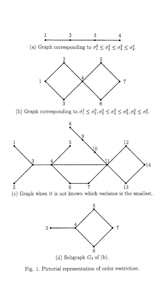
be applied to the estimation of each variance under various

types of order restrictions. Before proceeding any further, we introduce a

picto-tial notation of order restriction developed by Hwang and Peddada (1994). In

Fig 1, each graph $((\mathrm{a})-(\mathrm{d}))$ represents the corresponding order restriction. For

example Fig. 1 (a) correspondsto the simple order restriction$\sigma_{1}^{2}\leq 2\sigma_{2}^{2}\leq\sigma_{3}^{2}\leq\sigma_{4}^{2}$.

Note that $\sigma_{i}^{2}$’$\mathrm{s}$ are denoted by solid circles. We omit writing

$\sigma$ on the graphs

but only write the subscripts. If two circles are joined together by a line

seg-ment, it

means

that the circle with larger number is known to correspond to

the larger $\sigma^{2}$. For example Fig. 1 (b) corresponds to the order restriction

$\sigma_{1}^{2}\leq\sigma_{2}^{2}$,$\sigma_{3}^{2}\leq\sigma_{4}^{2}\leq\sigma_{5}^{2}$,$\sigma_{6}^{2}\leq\sigma_{7}^{2}$.

Now, we explain

an

improved estimation scheme. We should mention that

Hw ang and Peddada (1994) proposed similar procedure for estimating order

re-stricted location parameters of elliptically symmetric distributions. We first

con-sider the

case

when it is known which variance corresponds to the smallest

vari-ance ($\mathrm{e}.\mathrm{g}$. Fig 1 (a) and (b)). Without loss of generality, we assume that

$\sigma_{1}^{2}$ is the

smallest variance. The estimation procedure is given as follows.

Step 1. Estimation

_of

$\sigma_{1}^{2}$ From Theorem3.1 and Remark 3.2,we canconstruct

an isotonic regression estimator of$\sigma_{1}^{2}$ which gives the uniform improvement over

$V_{1}/w_{1}$ if$w_{1}$ is not solarge

as

shown in Theorem 3.1.

Step 2. Estimation

_of

other variances. When

we

estimate $\sigma_{l}^{2}$, we

remove

the

smallest number of circles from the graph sothat $\sigma_{i}^{2}$ becomes the smallest variance

in the resulting subgraph $G_{i}$. Then by Theorem $3.1_{\mathrm{I}}$

we can

construct an isotonic

regression estimator of $\sigma_{l}^{2}$ based on the circles in $G_{i\}}$ which gives the uniform

improvement

over

$V_{i}/w_{i}$ if$w_{i}$ satisfies the condition implied by Theorem 31.

Example. When we consider the estimation of $\sigma_{3}^{2}$ in Fig 1 (b), we

remove

the

circles 1

and

2 so that $\sigma_{3}^{2}$ corresponds to the smallest variance in the resulting

subgraph Fig 1 (d). We guess the unknown ordering between$\sigma_{5}^{2}$ and$\sigma_{6}^{2}$ inthe sub-graph $G_{3}$, and

we

havethe dummy simple order restriction $\sigma_{3}^{2}\leq\sigma_{4}^{2}\leq\sigma_{5}^{2}\leq\sigma_{6}^{2}\leq$

75

1234

(a) Graph corresponding to $\sigma_{1}^{2}\leq\sigma_{2}^{2}\leq\sigma_{3}^{2}\leq\sigma_{4}^{2}$

.

17

(b) Graph corresponding to $\sigma_{1}^{2}\leq\sigma_{2}^{2}$,$\sigma_{3}^{2}\leq\sigma_{4}^{2}\leq\sigma_{5}^{2}$,$\sigma_{6}^{2}\leq\sigma_{7}^{2}$

.

(c) Graph when it is not known which varianceis the smallest.

3 7

(d) Subgraph $G_{3}$ of (b).

$\sigma_{7}^{2}$. Then under this dummy order restriction,

we

construct isotonic regression

estimator of $\sigma_{3}^{2}$ based on $V_{i}/w_{i},$ $\mathrm{i}=3,4$,$\cdots$ ,7 with weights $w_{i}$, $\mathrm{i}=3,4$,$\cdots$ , 7,

that is $\hat{\sigma}_{3}^{2}s=\min_{3\leq j\leq k}[(\sum_{l=3}^{j}V_{l})/(\sum_{l=3}^{j}w_{l})])$ which gives the unifor$\mathrm{m}$

improve-ment

over

$V_{3}/w_{3}$ if$w_{i}$, $\mathrm{i}=3$,$\cdots$

}$7$satisfysome conditions. As for theestimation

of $\sigma_{2}^{2}$,$\sigma_{4}^{2}$,$\sigma_{5}^{2}$ and $\sigma_{6)}^{2}$ we can discuss similarly. However, our procedure does not

work for the estimation of$\sigma_{7}^{2}$, the largest variance.

When it is not known which variance corresponds to the smallest variance

(e.g. Fig 1 (c)), we

can

start with Step 2. We should notice here that though

our scheme gives improved estimators of each of order restricted variances, the

obtained estimates may violate the known order restriction unfortunately. To the

best of our knowledge, it is not well established when and how we can construct

such estimators which not only improve upon usual estimators but also preserve

the known order restriction.

3.2

Further improvement

Here, weshow that our improved estimator given in Section 3.1 can be further

improved upon uniformly by an estimator which usenot only $V_{i}’ \mathrm{s}$ but also $\overline{X}_{i}’ \mathrm{s}$

.

We give an estimator improving upon $\hat{\sigma}_{1}^{2^{S}}$

especially for the case when $k=2$

and $\sigma_{1}^{2}\leq\sigma_{2}^{2}$ is known. We

can

similarly discuss the estimation of each of order

restricted variances also for thhe case when $k\geq 3$

.

Let $Q_{j}=n_{j}\overline{X}_{j}^{2},\dot{\mathrm{J}}$ $=1,2$, then $Q_{j}’ \mathrm{s}$ are independentlydistributed as $\sigma_{j}^{2}\chi_{1}^{2}(\lambda_{j}))$where $\lambda_{j}=n_{j}\mu_{J}^{2}/(2\sigma_{j}^{2})$. We

can imagine random variables $Kj$, $j=1,2$ distributed independently as Poisson

distributions withmeans Xj, $j=1,2$such that given $K_{j}’ \mathrm{s}$, $Qj7s$

are

independently

distributed as $\sigma_{j}^{2}\chi_{1+2K_{j}}^{2}$ respectively. Further from Lemma 31 wc can imagine a

randomvariable$T_{2}$ such that$T_{2}$ given $K_{2}$ is distributed as $(\sigma_{2}^{2}-\sigma_{1}^{2})/(2\sigma_{1}^{2})\chi_{1+2K_{2}}^{2}$ and that $Q_{2}$ given $K_{2}$ and $T_{2}$ is distributed as $\sigma_{1}^{2}\chi_{1+2K_{2}}^{2}(T_{2})$. Thus, together with

the proof of Theorem 3.1, we can imagine auxiliary random variables $U_{2}$,$K_{1}$,$K_{2}$

and $T_{2}$ such that $V_{1}$, $V_{2}$, $Q_{1}$ and $Q_{2}$ given them are independently distributed as $\sigma_{1}^{2}\chi_{\nu_{1}}^{2})$ $\sigma_{1}^{2}\chi_{\nu_{2}}^{2}(U_{2})$, $\sigma_{1}^{2}\chi_{1+2K_{1}}^{2}$ and $\sigma_{1}^{2}\chi_{1+2K_{2}}^{2}(T_{2})$. Note that

$\hat{\sigma}_{1}^{2}s$

is expressed as

$\min\{a_{1}V_{1}, a_{2}(V_{1}+V_{2})\}$, (23)

where $a_{\underline{1}}$ and $a_{2}$ are given constants. Alsonote thatwhen we considerthe

estima-then of $\sigma^{2}$ under entropy loss (or squared

error

loss),

$a_{1}$ and $a_{2}$ must satisfy the

condition $a_{1}>a_{2}\geq 1/(\nu_{1}+l/_{2})$ (or $a_{1}>a_{2}\geq 1/(lJ1+\iota\prime_{2}+2)$). Similarly with the

proof of Theorem 3.1, we see that $\hat{\sigma}_{1}^{2^{S}}$

is improved upon uniformly by

$\min\{a_{1}V_{1}, a_{2}(V_{1}+V_{2}), a_{3}(V_{1}+V_{2}+Q_{1}), a_{4}(V_{1}+V_{2}+Q_{1}+Q_{2})\}$ (24)

if$a_{j}\geq 1/(\nu_{1}+l/_{2}+j-2)$ and $a_{j-1}>a_{\mathrm{i}}$, $j=3,4$ (or if $a_{j}\geq 1/(\nu_{1}+\nu_{2}+j)$ and

77

We should mention that we

can

construct an estimator $\mathrm{i}$mproving upon _{$a_{1}V_{1}$}

by using Vi, $V_{2}$, $Q_{1}$ and $Q_{2}$ regardlessof the pooling order of $V_{2}$, $Q_{1}$ and$Q_{2}$

.

For

example$\mathrm{J}$

rrnn{

$a_{1}V_{1},$$b_{2}(V_{1}+\mathrm{Q}2),$$b_{3}$($V_{1}+Q_{1}+\mathrm{V}2$ _,a$\{\mathrm{V}\mathrm{i}+Q_{1}+V_{2}+Q_{2}$)$\}$ (25)

and

$\min$

{

$\mathrm{a}\{\mathrm{V}\mathrm{i} c_{2}(V_{1}+Q_{2}), \mathrm{c}_{3}(V_{1}+Q_{2}+Q_{\mathrm{J}} ), c_{4}(V_{1}+Q_{2}+Q_{1}+V_{2})\}$ (26)

uniformly improve upon $\mathrm{a}\mathrm{i}$Vi if

$a_{1}$, $b_{j}$, $j=2,3,4$ and

$c_{j}$, $j=2,3$,4 satisfy some

conditions which will be apparent from Theorems 2.2 and 2.3.

References

[1] Barlow, R. E., Bartholomew, D. J. Bremner, J. M. and Brunk, H. D. (1972).

Statistical Inference under Order Restrictions: The Theory and Application

ofIsotonic Regression. Wiley, New York.

[2] Brew ster, J. F. and Zidek, J. V. (1974). Improvingonequivariantestimators.

Ann. Statist. 2, 21-38.

[3] Brown, L. (1968). Inadmissibility ofthe usual estimators of scaleparameters

inproblemswithunknownlocation and scale parameters. Ann. Math. Statist.

39, 29-48

[4] Gelfand, A. E. and Dey, D. K. (1988). Improved estimation of the disturbance

variance in a linear regression model. J. Econometrics 39, 387-395

[5] Hwang, J. T. (1985). Universal domination and stochastic domination:

es-timation simultaneously under a broad class of loss functions. Arm. Statist.

13, 295-314.

[6] Hwang, J. T. G. and Peddada, S. D. (1994), Confidence interval estimation

subject to order restrictions. Ann. Statist. 22,

67-93.

[7] Nagata, Y. (1989). Estimation with pooling procedures of

error

variance in

ANOVA for orthogonal arrays. J. Jap. Soc, _{Quality Control} 19, 12-19. (in

Japanese. )

[8] Oono, Y. and Shinozaki, N. (2004). Estimation oferror variance in the

anal-ysis ofexperiments usingtwo-level orthogonal arrays. Comm. Statist. Theory

Methods 33, 75-98.

[9] Robertson, T., Wright, F. T. and Dykstra, R. L. (1988). Order Restricted

[10] Shinozaki, N (1995). Some modificationsof improved estimators of anorm al

variance. Ann. Inst. Statist. Math. 47,

273-286.

[11] Stein, C. (1964). Inadmissibility ofthe usual estimator for the variance of a

normnal distribution with unknown mean. Ann. Inst. Statist. Math, $16_{7}155-$