On a free boundary problem related to the motion of an amoeba (Nonlinear evolution equations and related topics to mathematical analysis of a phenomena)

(1)

On

a free

boundary problem

related to

the

motion

of

an

amoeba

Harunori Monobe

Mathematical

Institute,

Tohoku

University

1 Introduction

Amoeba motion is

one

of cellular motions. and is common among many cells. for

example, white blood cell,

cancer

cells, slime mold, keratocyte and so on. The

locomotionis caused by

some

chemical reactions within acell and substances outside

the cell. However the detailed mechanism to produce such motion structure is not

well understood so that its mathematical study is an interesting question.

Meanwhile, there are some mathematical models proposed by a lot of biologist

and physicist who desire to understand thelocomotion. In this paper we consider a

mathematical model. which is proposed by T. Umeda [6], of them.

We consider the following free boundary problem:

(P) $\{\begin{array}{ll}u_{t}=\triangle u+k_{1}(C_{0}-\int_{\Omega(t)}udx)-u+k_{2} in Q. \cdot\cdot\cdot (i)u=1+A\kappa+BV on \Gamma, \cdots(ii)V=-\epsilon\nabla u\cdot n+g(C_{0}-\int_{\Omega(t)}udx)-u on \Gamma, \cdots(iii)u=\phi\geq k_{2} in \Omega(0),\end{array}$

where $\Omega(t)$ is anunknown bounded domain in$\mathbb{R}^{2}$ at time

$t$ with the boundary$\partial\Omega(t)$,

$Q$ and $\Gamma$

are a

non-cylindrical

domain and

a

non-cylindrical surface, respectively.

defined by

$Q:= \bigcup_{t>0}\Omega(t)\cross\{t\}_{\dot{\pi}}$ $\Gamma:=\bigcup_{t>0}\partial\Omega(t)\cross\{t\}$,

$\kappa=\kappa(x, t)$ is an inward curvature at $x\in\partial\Omega(t),\cdot V=V(x, t)$ is a scalar function

representing the outer normal velocity of$\partial\Omega(t),$ $n=n(x, t)$ is anouter normal unit

vector at $x\in\partial\Omega(t)$. Coefficients $k_{1},$ $k_{2},$$C_{0}$,A.$g$

are

positive constants and B.$\epsilon$ are

non-negative constants.

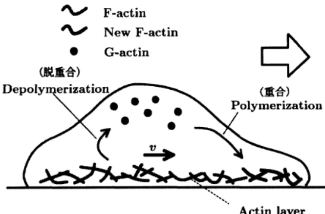
(P) is related to a mathematical model describing the motion of an amoeba,

which is based on the density of F-actin $u(x, t)$ and actin layer $\Omega(t)$ contained in a

(2)

$\sim$ _F-actin

Actin layer

Figure 1:

Cross

section of

a

cell

can

regard the domain

as

the shape ofthe cell.

Onthe otherhand, (P) is regarded mathematicallyas aone-phaseStefan problem

with reaction terms. In terms of Stefan problems, the interior condition (i) and

boundary conditions (ii), (iii) correspond to the heat equation, the Gibbs-Thomson

effect and the

Stefan

condition, respectively. Ingeneral, for free boundary problems,

the topoloy

of domains may

change at

a

finite time

so

that the existence time

of

classical solutions is local. Therefore,

some

additional conditions

are

necessary for

the existence ofthe time global classical solutions. In what follows,

we

consider the

time local and time global existence ofsolutions for (P) under some assumptions.

Assumption 1. The initial domain $\partial\Omega(0)\dot{h}9$ a Jordan

curve

such that $\partial\Omega(0)\in$

$C^{3+a},$ $\partial\Omega(0)=\{X^{0}(s)+\Lambda_{0}(s)N(s)|s\in[0, l]\}$ , where $\alpha$ is a Holder index $(0<$

$\alpha<1),$ $X^{0}$ is a regular Jordan curve, in $\mathbb{R}^{2}$, parameterized by

$s$

.

Here $N(s)$ is the

outer nomal unit vector at $X^{0}(s)$, and $\Lambda_{0}\in C^{3+\alpha}([0, l])$.

Definition 1. In the

case

_of

$\epsilon>0$, we call (P) has

a

time local solution”,

if

there

exists

a

_finite

time $T>0$ such that $(u, \Omega(t))$

satisfies

(P) and have a regularity

$u\in C^{2+\alpha,(2+\alpha)/2}(\overline{Q_{T}})$, $\Gamma_{T}\in C^{3+\alpha,(3+\alpha)/2}$,

where $Q_{T}= \bigcup_{0<t<T}\Omega(t)\cross\{t\}$ and $\Gamma_{T}=\bigcup_{0<t<T}\partial\Omega(t)\cross\{t\}$

.

Also,

if

$T=\infty$, we

call “(P) has a unique time globalsolution ”.

Considering the viscosity effect $(B>0)$,

we

have the following result:

Theorem 1. Let$B,$$\epsilon>0$. Suppose that$\partial\Omega(0)$

satisfies

Assumption 1.

If

the initial

datum$\phi$ belongs to $C^{2+\alpha}$(St(0)) and

satisfies

a

compatibility condition, then (P) has

a unique time local classical solution.

In Theorem 1,

as

in X. Chen and F. Reitch [1], W. Merz and P. Rybka [4],

we

regard the boundary condition (ii)

as a

parabolic problem

on a

curve, and

an

approximate sequence of the boundary

can

be found by solving the problem. As

a

result,

we

have

a

unique solution with the aid of the Hanzawa diffemophism (E.

Hanzawa [2]$)$ and Banach$s$ fixed point theorem. On the other hand, in the

case

of

(3)

an approximate sequence of the boundary with the time evolution. However, under

the special condition (spherically symmetric case). we can show the existence of

classical solutions since we

can

construct an approximate sequence of the boundary

by the boundary condition (iii). From now on, we consider the case where $(\phi, \Omega(0))$

is spherically symmetric.

Assumption 2. Initial data are spherically symmetric, $i.e$.

$\Omega(0)=\{x\in \mathbb{R}^{2}|0\leq|x|<s_{0}\}$, $\phi(x)=\psi(|x|)$.

where $s_{0}$ is apositive constant and $\psi\in C^{2+\alpha}([0.s_{0}])$ with $\psi_{r}(0)=0$.

From now on, we suppose that initial data satisfy Assumption 2.

Definition 2. In the case

_of

$\epsilon=0$, we call “(P) has a time local classical solution“,

if

there exists $T>0$ such that $(u, \Omega(t))$

satisfies

(P) and have a regularity

$u\in C^{2+\alpha\prime}(2+\alpha)/2(\overline{Q_{T}})$, $\Gamma_{T}\in C^{4+\alpha.(4+\alpha)/2}$.

Also,

_if

$T_{*}=$ oo, we call “(P) has a unique time global solution “.

Theorem 2. Let $B=0$ and $\epsilon\geq 0$.

If

the initial datum $\phi$

satisfies

Assumption 2

and compatibility conditions, then (P) has a unique time local classical solution.

From the viewpoint of mathematical modeling, it is preferable that $u$ and $C_{0}-$

$\int_{\Omega(t)}udx$are positive. With this view in mind, weconsider the time global existence

of solutions in the case of$\epsilon=0$.

Assumption 3.

_Coefficients

satisfy the following condition:

$k_{1}C_{0}-(1-A\pi g)(1-k_{2})<0$. $1-k_{2}>0$.

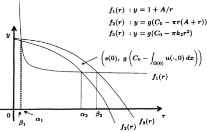
Assumption 4. There exists $\alpha_{1},$$\alpha_{2},$$\beta_{1}.\beta_{2}\in(0, (-A+\sqrt{A^{2}+4C_{0}}/\pi)/2]$ such that

following conditions hold:

$g(C_{0}- \pi\alpha_{i}(A+\alpha_{i}))=1+\frac{A}{\alpha_{i}}$, $g(C_{0}- \pi k_{2}\beta_{i}^{2})=1+\frac{A}{\beta_{i}}$, $(i=1,2)$.

where $\alpha_{1}<\alpha_{2}$ and$\beta_{1}<\beta_{2}$.

Theorem 3. Let $B=0$ and$\epsilon=0$. Suppose that initial data and

coefficients

satisfy

Assumption 2, 3,

_{4. If}

initial data satisfy compatibility conditions and

$k_{2}<\phi|_{\Omega(0)}<\phi|_{\partial\Omega(0)}$, $C_{0}- \int_{\Omega(0)}\phi dx>0$, $\alpha_{2}\leq s_{0}\leq\beta_{2}$,

then (P) has a unique time global solution $(u, \Omega(t))$ such that

$k_{2}<u|_{\Omega(t)}<u|_{\partial\Omega(t)}$. $C_{0}- \int_{\Omega(t)}u(t, \cdot)dx>0$, $\alpha_{2}\leq s(t)\leq\beta_{2}$,

(4)

2 Positive

invariant

region

Local existence of

a

classical solution for (P) is shown by Hanzawa diffe.[2],

a

parabolic standard existence theory [3] and $Banach\prime s$ fixed point theorem (see [5]).

The proof is based on the paper ofChen and Reitch [1].

In this section.

we

prove the existence of a positive invariant region, for $\partial\Omega(t)$,

to show the existence of a time global classical solution. To this end,

we

examine

some

properties such that

$\phi>k_{2}(>0)$, $C_{0}- \int_{\Omega(0)}\phi dx>0\Rightarrow$ $u>k_{2}$, $C_{0}- \int_{\Omega(t)}udx>0$.

These properties

come

from the fact that

area

densityof F-actin and concentration

of G-actin are positive in the biological view point. Likewise, they

are

of help to

prove the boundedness of $u$ and $\Omega(t)$. As

a

result. we

can

find global solutions with

the help ofthese properties and initial conditions.

Here, for simplicity,

we

rewrite (P) as

an

one-dimensional problem

(SP) $\{\begin{array}{ll}v_{t}=v_{rr}+\frac{v_{r}}{r}+k_{1}(C_{0}-2\pi\int_{0}^{s(t)}rvdr)-v+k_{2} in Q((0, T);s(t)),v=1+\frac{A}{s(t)} on \Gamma((0.T);s(t)),\dot{s}(t)=g(C_{0}-2\pi\int_{0}^{s(t)}rvdr)-v on \Gamma((0.T);s(t)),v_{r}=0 on \{0\}\cross[0, T],v=\psi>k_{2} in (0, s_{0}),\end{array}$

where $T$ is a positive constant,

$Q((a.b);s(t)):= \bigcup_{a<t<b}[0, s(t))\cross\{t\}$, $\Gamma((a, b);s(t)):=\bigcup_{a<t<b}\{s(t)\}\cross\{t\}$

and $v(r, t)$ is equal to $u(x, t)$ for (P) with _$r=|x|$.

2.1 Boundedness

of

$s(t)$

and

$v(r, t)$

To prove Theorem 3, we prepare some Lemmas. From

now

on,

we

suppose that $T$

is a time such that (SP) has the unique time local solution $(v, s(t))$ in $[0, T]$.

Lemma 1. Assume that $\dot{s}(t)\leq 0$

for

any $t\in[t_{0}, t_{1}]\subset[0, T]$

.

If

$k_{2}<v(r, t_{0})<$

$v(s(t_{0}), t_{0})$

for

any $r\in[0, s(t_{0}))$ and $C_{0}-\pi(A+s(t_{0}))s(t_{0})>0$, then

$k_{2}<v(r, t)<v(s(t).t)$, $C_{0}-2 \pi\int_{0}^{s(t)}rvdr>0$

(5)

Proof.

It is clear in the

case

of$t_{0}=t_{1_{\dot{}}}$

so we

consider the

case

of$t_{0}\neq t_{1}$. Suppose

that there exists a point $(r^{*}, t^{*})\in Q((t_{0}. t_{1}];s(t))$ such that $v(r^{*}, t^{*})=k_{2}$ and $k_{2}<$

$v(r.t)<v(s(t), t)$ _in $Q((t_{0}.t_{1});s(t))$. where $Q((a.b];s(t))$ $:= \bigcup_{a<t\leq b}[0.s(t))\cross\{t\}$.

Since $\dot{s}(t)\leq 0$ and $v\leq v(s(t), t)$ for $t\in[t_{0}, t^{*}]$,

$C_{0}-2 \pi\int_{0}^{s(t)}rvdr>C_{0}-\pi(A+s(t))s(t)>C_{0}-\pi(A+s(t_{0}))s(t_{0})>0$_.

Then, from the interior condition of (SP),

$0\geq v_{t}(r^{*}, t^{*})$

$=v_{rr}(r^{*}.t^{*})+ \frac{v_{r}(r^{*},t^{*})}{r}*+k_{1}(C_{0}-2\pi\int_{0}^{s(t^{*})}rvdr)-v(r^{*}.t^{*})+k_{2}>0$.

This is

a

contradiction. and we

see

that $v>k_{2}$ for $t\in[t_{0}.t_{1}]$. On the other hand,

suppose that there exists a point $(r^{*}, t^{*})\in Q((t_{0}, t_{1}];s(t))$ such that $v(r^{*}, t^{*})=$

$1+A/s(t^{*})$ and _{$k_{2}<v(r, t)<1+A/s(t)$} in $Q((t_{0}, t_{1});s(t))$. From easycalculations,

$C_{0}-2 \pi\int_{0}^{s(t)}rvdr$ and $\int_{0}^{s(t)}rvdr$ are positive for $t\in[t_{0}.t^{*}]$. Then

$0 \leq v_{t}(r^{*}, t^{*})\leq k_{1}C_{0}-2k_{1}\pi\int_{0}^{s(t^{*})}rvdr-(1-k_{2})-\frac{A}{s(t^{*})}<0$

from Assumption 4. This is a contradiction, and we see that $v<v(s(t), t)$ for

$t\in[t_{0}, t_{1}]$.

$\square$

Similarly. for the

case

of $\dot{s}(t)\geq 0$. we will show the boundedness. Here we

remarkthat the assumption of boundedness for $s(t)$ differ slightly between $\dot{s}(t)\geq 0$

and $\dot{s}(t)\leq 0$.

Lemma 2. Assume that $\dot{s}(t)\geq 0$

for

$t\in[t_{0}, t_{1}]\subset[0.T]$, and $s(t_{0})\geq\alpha_{2}$.

If

$k_{2}<v(r, t_{0})<v(s(t_{0}), t_{0})$

for

any $r\in[0, s(t_{0}))$ and $C_{0}-\pi(A+s(t_{i}))s(t_{i})>0$

for

$i=0_{:}1$, then

$k_{2}<v<v(s(t).t)$, $C_{0}-2 \pi\oint_{0}^{s(t)}rvdr>0$

for

any $t\in[t_{0}, t_{1}]$ and _{$r\in[0.s(t))$}.

Proof.

We show this Lemmainthecaseof$t_{0}\neq t_{1}$ only. Fromthe boundary condition

(iii) and $\dot{s}(t)\geq 0$, it follows that $C_{0}-2 \pi\int_{0}^{s(t)}rvdr>0$ for any $t\in[t_{0}, t_{1}]$. As the

argument ofLemma 1, we have the property $v>k_{2}$. To prove that $v<v(s(t), t)$ in

$(0, s(t))$. we use

a

_{super-solution} $1+A/s(t)$.

Let$X(r, t)=1+A/s(t)-v(r, t)$. From directly calculations, $X(r.t)$ satisfies the

following problem:

$\{\begin{array}{ll}X_{t}=X_{rr}+\frac{X_{r}}{r}-k_{1}(C_{0}-2\pi\int_{0}^{s(t)}rvdr)-X -k_{2}+(-\frac{A\dot{s}(t)}{s^{2}(t)}+1+\frac{A}{s(t)}) in Q((t_{0}, t_{1});s(t)),X(s(t), t)=0.X_{r}(0, t)=0, X(r,\cdot 0)\geq 0 in (0, s_{0}).\end{array}$

(6)

Figure 2: Assumption 4

Suppose that there exists a point $(r^{*}, t^{*})\in Q((t_{0}, t_{1}];s(t))$ such that $X(r^{*}, t^{*})=0$

and $X(r.t)>0$ in $Q((t_{0}.t^{*});s(t))$

.

The left hand side $X_{t}(r^{*}, t^{*})\leq 0$. On the other

hand, since $\dot{s}(t)\geq 0,$ $s(t_{0})\geq\alpha_{2}$ and $C_{0}-\pi(A+s(t_{1}))s(t_{1})>0$,

$0 \leq g(C_{0}-2\pi\int_{0}^{s(t)}rvdr)-1-A/s(t)$

$<g(C_{0}-2 \pi\int_{0}^{s(t)}rvdr)-g(C_{0}-\pi s(t)(A+s(t)))$ (2)

for any $t\in[t_{0}, t_{1}]$ (see Figure 2). Moreover, by normalizing free boundary,

$2 \pi\int_{0}^{s(t)}rvdr>k_{2}\pi s^{2}(t)$ (3)

for any $t\in[t_{0}, t_{1}]$, where $v(r, t)=w(\rho, t)$ and $r=\rho s(t)$. By (2), (3) and Assumption

3, we see that

$\{-k_{1}(C_{0}-2\pi\int_{0}^{s(t)}rvdr)+1-k_{2}\}s^{2}(t)$

$+A \{s(t)-g(C_{0}-2\pi\int_{0}^{s(t)}rvdr)+1+A/s(t)\}$

$>\{-k_{1}C_{0}+(1-Ag\pi)(1-k_{2})\}s^{2}(t)+A(1-Ag\pi)s(t)>0$.

Hence we

see

that the right hand side of interior condition is positive at the point

$(r^{*}, t^{*})$

.

This is a contradiction for the assumption of $(r^{*}, t^{*})$, and we have the

Lemma. $\square$

Remark 2.1. Assumption

₄

just

means

that, in Figure 2, $f_{1}(r)$ and$f_{2}(r)$ have two

intersections in the interval $(0, r_{*})$, where $f_{2}(r_{*})=0$. This relation

of

$f_{1}(r)$ and

(7)

Figure 3: Cross section ofa cell

Rom these Lemmas 1, 2, we see that

$\alpha_{2}\leq s(t)\leq\beta_{2}$

.

Lemma 3. Initial data satisfy following conditions:

$k_{2}<\psi|_{[0,so)}<\psi(s_{0})$, $\alpha_{2}\leq s_{0}\leq\beta_{2}$, $C_{0}-2 \pi\int_{0}^{s_{0}}r\psi dr>0$,

then

$k_{2}<v<v(s(t), t)$. $\alpha_{2}\leq s(t)\leq\beta_{2_{\dot{\text{ノ}}}}$ $C_{0}-2 \pi\int_{0}^{s(t)}rvdr>0$,

for

any $t\in[0, T]$ and $r\in[0, s(t))$.

By using the result of boundedness for $u$ and $s(t)$, we obtain the boundedness

for the H\"older norm of $s(t)$, As a result, we have the exsictence of the time global

solution for (P). Here

we

remark that the profile of$u$ is that the value in a

neigh-borhood of the boundary is larger than one of the inside (see Figure 3). Actually,

we can make sure of the truth that there exists some livin$g$ things such that the

density of F-actin in the cell is similar to the solution for (P).

Acknowledgment

The author would like to thank Prof. Toyohiko Aiki for giving me an opportunity

to have a talk in this RIMS workshop, “Nonlinear evolution equations and related

topics to mathematical analysis of phenomena” Also I want to thank Prof. Eiji

Yanagida for encouraging the author to analyze this problem and several helpful

comments, and Professor Tamiki Umeda for valuable suggestions to this biological model.

(8)

References

[1] X. Chen and F. Reitch, Local existence and uniqueness ofthe stefan problem

with surfacetension and kinetic undercooling, J. Math. Anal. Appl. 164 (1992),

350-362.

[2] E. Hanzawa, Classical solution of stefan problem, Tohoku Math. J. 33 (1981).

297-335.

[3] O. A. Lady\v{z}enskaja, V. A. Solonnikov

and

N. N. Ural‘ceva, Linear and

quasi-linear equations of parabolic type, Traslations of mathematical monographs

Amer. Math. Soc, Providence, R. I, 1968.

[4] W. Merz and P. Rybka, A free boundary problem describing

reaction-diffusion

problem in

chemical

vapor

infiltration

of pyrolyticcarbon, J. Math. Anal. Appl.

292 (2004), 571-588.

[5] H. Monobe, Existence of solutions for a mathematical model related to the

motion of an amoeba, to appear, in Adv. Math. Sci. Appl. 2 of Vol. 20 (2010).

[6] T. Umeda, A chemo-mechanical model for amoeboid cell movement (in