Estimation in a Mixed Proportional Hazards Model (Mathematics and Algorithms of Optimization)

Estimation in

aMixed

Proportional

Hazards Model

JONG WOON KIM

Department of IndustrialEngineering,Pusan National University, San30Changjeon-DongKumjeong-Ku,

Busan ,609-735,KOREA

timer\copyright pusan.ac.kr

WONYOUNG YUN

Departmentof Industrial

Engineering,

PusanNational University, San

30

Changjeon-Dong Kumjeong-Ku,

Busan,609-735,KOREA

wonyun\copyright pusan.ac.kr

TADASHIDOHI

Department Information Engineering,Graduate Schoolof Engineering, Hirosima University, 1-4-1

Kagamiyama, Higashi-Hirosima739-8527,JAPAN

dohi\copyright rel.hiroshima-u.ac.jp SUMMARY

Cox’s proportional hazards model (PHM) has been widely applied in the analysis of lifetime data, and

can

be

characterized by covariates influencing lifetime of asystem, where the

covariates

describe operating

environments (e.g. temperature,

pressure,

humidity). When environments

are

uncertain, the

covariates may

be

oftenmodeled

as

randomvariables.We

assume

that

acovariate

isadiscrete randomvariable,and

propose

anew

mixture type ofPHM, called the mixed PHM. We develop the Expectation-Maximization(EM) algorithm to

estimatethe model parameters. Two types ofobservations

are

considered;

one

type of observations is obtained

ffom experimentalunits,which

are

tested in laboratories and the othertypeofobservations

is

obtained ffom field

unitswhich

are

operated by customers. An illustrative exampleis given.

Keywords:Proportional hazardsmodel,Mixturemodel, Estimation,EMalgorithm,Failure data analysis.

1. Introduction

Notation

$s$ :random variable of

acovariate

$s_{k}$ :the$h\mathrm{h}$element of

acovariate

$g$ :thenumber of elements$\mathrm{o}\mathrm{f}s$

数理解析研究所講究録 1297 巻 2002 年 169-178

$n$ :the numberof uncategorized field

units

$m_{i}$ :the number categorized experimental unitswhosecovariates

are

$s_{i}$

$m_{sum}$

:

$\sum_{j=1}^{g}m_{i}$

$x_{j}$ :thefailure time of theyth uncategorized unit.

$y_{j},\cdot$ :thefailuretime oftheythunit

among

the categorizedunitswhosecovariates

are

$s_{j}$

.

$\theta$ :avector lifetime

distribution

parameters.

$\eta$ :avectorofaregressionparameter

$\emptyset$

:

$(\eta,\theta)$

$\psi$

:

$(\mathrm{p},\eta,\theta)$

An importantproblemin the failure dataanalysis

is

that all partsofthe data have not always beencollected

under similar conditions. For example,

we

often encounter the

situation

where apiece of equipment

may

have been used in different environments

or may

have adifferent

age

or

modification status. Such different

environments will affect the equipment’s inherent reliability characteristics obviously. Therefore, it

may

be

useffiltotake accountofthe environmentalfactors in equipment reliability modeling. The proportional hazards

model (PHM), which

was

proposed by Cox, has been considered

as

auseffil tool to deal with environmental

factors in the analysis of lifetime data. Solomon[17] indicated that significanteffects for

covariates

would be

obtained

even

inthe

cases

where themodel

was

notwhollyappropriate,and showed that the PHM

is

relatively

robust to departures ffomthe proportional hazards assumption. The applicationofPHM to reliabilitydata has

been considered by anumber ofauthors, for example, Ansell&Phillips[l] and Jozwiak[8]. Foralistof

more

recentpapers,

see

thereview

paper

byKumar andKlefsj6[10].

Let$T$beanon-negativerandomvariable and denote the failuretimeof

an

item under consideration.

Thefailurenature this

item

can

be modeled bythehazardrate $\lambda(t)$

:

$\lambda(t)=\lim_{harrow 0}\frac{P(t\leq T<t+h|T\geq t)}{h}$

(1)

Theassumption inthe PHM, in most cases, is thatthehazardrateofasystemisthe productof

an

arbitrary and

unspecified baseline hazard rate $\lambda_{0}(t)$ depending

on

only time, andapositiveffinctional term $\omega(s;\eta)$,whichis

basically independent oftime. The function $\omega(s;\eta)$ is introduced to incorporate the effects ofanumber of

covariatessuch

as

temperature,

pressure

and changes in design.Thus,thehazard rateinthe PHMis givenby

$\lambda(t;s)=\omega(s;\eta)\lambda_{0}(t)$ (2)

where $s$ is

arow

vector consisting ofthe

covariates

and $\eta$ is acolumn vectorconsisting ofthe regression

parameters. The reliability ffinction and the densityffinction inthegenericPHM

are

given by

$R(t;s)=\exp[-\mathrm{J}$$\lambda_{0}(u\mathcal{M}s;\eta \mathrm{W}u]$ (3)

$f(t;s)=\lambda(t;s)R(t;s)$ ₍₄₎

Therearetwowaystomodel the baseline hazardrate $\lambda_{0}(t)$;parametricmodel andnon-parametricmodel. Inthe

parametric model,

we assume

asuitable theoretical distribution for $\lambda_{0}(t)$. On the other hand, in the

non-parametric model,

no

specific distribution is assumed. Note that the non-parametric method cannot always

guarantee

an

accurate

estimation

becauseofthe lackofknowledge

on

the lifetimedistribution. InthisPaPer,two

representativelifetime distributions; the exponential and the Weibull distributions,

are

assumedfor $\lambda_{0}(t)$. It is

also assumed in

many

cases

that thefunctional form of $\mathrm{a}\langle s;\eta$

)

isknown. Varioustypes of functional forms of

$a \int s;\eta$$)$ havebeenproposed inthe past literature. Someofthese

are:

theexponentialform, $\exp(s\eta)$;thelogistic

form, $\log(1+\exp(s\eta))$;the inverse linear form,

l/(l+s\eta );

and the linear form, $1+s\eta$ . In this

paper,

we

assume

the exponential form which has been most widelyused in applications. Covariates

are

associatedwith

the equipment’s environmental and operational conditions and $\eta$ is the effects of thecovariates.

We consider

asituation

where equipment’senvironmental and operational conditions

are

various.

In Martorell,

Sanchez&Serrade11,[12], it

was

reported that theequipmentat nuclear

power

plants works under

very

different

operating conditions. In addition,

very

different environmental conditions

appear

in anuclear

power

plant. That

is,

some

components

are

placed in

avery

hardenvironment, for instance, under high temperatureand dosesof

radiation, while others

remain

in acomfortable environment. Insuch acase, the

covariates

can

be modeled

as

variables. Also,

we

cannot figure out theconditionunderwhich aproduct is operated before installing it. These

variability anduncertaintyofthe

covariates

make

us

considerthe

covariates

as

random variables.

For notational and computational convenience, suppose that the number ofthe covariates for

one

unit, is only

one.

Define the probability

mass

function oftherandom covariate$s$by

$p_{1}$ $p(s)=$

.

$\cdot$

.

$-p_{g}$ when $s=s_{1}$

...

(5) when $s=s_{g}$

It

is

assumed in this

section

that thesupportofthe randomvariable,$s$, isknown.

Underthese assumptions, theprobability density function of the

time

to failure is represented inthe following

finitemixtureform,

$f(t)= \sum_{-i1}f(t,s_{i})=\sum_{i-=1}p_{i}f(t;s_{i})=\sum_{i_{-}^{-}1}p_{i}\lambda_{0}(t\mu_{s_{i};\eta})\exp[-\int h$

(

$u\ltimes\{s_{i};\eta \mathrm{k}^{y}]$ (6)

The mainpurposeof this article istoestimate lifetime distributions of the products whose failures phenomena

can

be modeled by themixedPHM. We

assume

that data

are

collectedffom two types ofobservations;

one

tyPe

of observations is obtained from experimental units, which

are

tested at laboratories and the other tyPe of

observations is obtained ffomfield

units

which

are

operatedby customers. Itisalsoassumedthatthe

covariate

of

an

experimental

unit

is known before testing and

so

$m_{i}$’s

are

constant;however,for afield

unit

we

don’tknow

the valueofthe

covariate

butknow the supportofit’s discreteprobability

mass

ffinction.

It represents thereal-world conditionthatproducts

are

tested in laboratoriesunderall possiblestress levelsofthe

real fields. For

an

example ofair-conditioners, they might be testedundervarioustemperatures at laboratories.

The assumption that the support ofthe

covariate

is known, describes that atemperature under which asold

product is operated is

one

among temperatures under which products

are

tested at laboratories. Generally

temperatures

can

be controlled at laboratories, and

so we

can

know it for each air-conditioner. However, it is

verydifficult toinvestigatethe temperatureforeveryair-conditioner failedat fields,and

so

we

maynotknow the

temperaturesforfieldunits.

With these two types of observations,

we

develop maximum likelihood techniques of model parameters;

distributionparameters,

mixing

proportions and aregressionparameter,based

on

theEMalgorithm.

ThemixedPHMis akind of

mixture

model. Theextensive applicability ofthemixed distributionshas generated

many

research problems. The existing results for estimating model parameters

in

the

mixture

model

were

classifiedandintroduced byTitteringtonet$\mathrm{a}1[19]$,Everitt&Hann[2], and

McLachlan&Basford[14].

The finite

mixed exponential distribution and thefinitemixed Weibulldistribution

are

goodcandidates to representfailure

times. McClean[13] considers the fitting ofmixed exponential distribution to the groupedfollow-up data when

the numberof componentsis known.Lau[ll]estimateshazard rate inbothmixture of geometries and mixture of

exponentials model. Jiang &Kececioglu[6] and Jiang &Murthy[5]

use

graphical approaches and Jiang

&

Kececioglu[7]

propose maximum

likelihood estimates(MLE) ffom censored data for

estimation

of the mixed

Weibull distributions. Jaisingh et $\mathrm{a}1[4]$ considere the

influence

of the work

environment using

aWeibull

&

inverse

Gaussian mixture. Hirose[3] deals withthe power-law mixture model which extendsthe

power

law in

accelerated life testing. Sy &Taylor[18] and Peng

&Dear[16]

involve the

mixture

models in PHM for

estimating

cure

rate. They assumed

no

specific theoretical

distribution

forthe baseline hazardffinctionand

use

twonon-parametric mixture models.

2. Estimation.

2.1 MaximumLikelihoodEstimation

Inthis

section

we

introduce the

maximum

likelihood method for estimatingparametersof the mixed proportional

hazards model.Notonlyis it appealing

on

intuition

grounds,butit also

possesses

desirable statistical properties.

Forexample, under

very

general conditionsthe

estimators

obtained by the method

are

consistent

and they

are

asymptoticallynormallydistributed

As mentionedbefore,

we

consider both the observations in laboratoriesandthe observations in field. Both of

them

are

incomplete, because the values of the covariates

are

missed in field units and it is impossible to

estimatethe mixing proportions usingobservations ffomonlyexperimental

units.

Consider asampleconsisting

of both$n$independentfield unitsand $m_{sum}$ independent experimentalunits.

Theobserved fulllikelihood ffinctionfor this sampleis defined by

$L( \psi)=\prod_{i\overline{-}1}^{n}\sum_{j\overline{-}1}p_{j}f(x_{j}$;$s_{j}, \phi)\cross\prod_{i\overline{-}1}\prod_{j\overline{-}1}^{m}’ f(y_{ij}$;$s_{j},\phi)$ (7)

The problem is toobtain the estimates $\hat{\psi}$ whichmaximize$L(\psi)$

.

However, it is not

easy

tofindthe MLEs in

the traditional

way

ofdifferentiating$L$ with respect to

$\psi$and setting itequal to zero, because the likelihood

ffinction often becomes acomplex multi-modal ffinction. An

alternative way

isto aPPly

an

iterative

algorithm

such

as

the EM algorithm.

Theestimate of $p_{k}$

can

be calculated by the similar methodto the generic mixture distributions. To

maximize

thislikelihoodsubject totheconstraint, $\sum p_{k}=1$,

we

introduce aLagrange multiplier and

maximize

$\log L(\psi)=\sum_{i=1}^{n}\log(\sum_{j=1}^{g}p_{j}f(x_{i};\phi,s_{j}))+\sum_{i=1}^{g}\sum_{-,j-,1}^{m}’\log f(y_{ij};\phi,s_{i})-\gamma(\sum_{i=1}^{g}p_{i}-1)$ (8)

Thisyields

$\frac{\partial 1\mathrm{o}\mathrm{g}L(\psi)}{\delta p_{k}}=\sum_{i=1}^{n}(f(x_{i};\phi,s_{k}/)\sum_{j=1}p_{j}f(x_{i};\phi,s_{j}))-r=\sum_{-i-1}^{n}(f(x_{i};\phi,s_{k})/f(x_{i}))-\gamma=0$ (9)

The Lagrange multiplier, $\gamma$,

can

be founded bymultiplying (9)by $p_{k}$ andsumming

over

$\mathrm{k}$togive $n-\gamma=0$

.

Theposterior probabilitythat the

covariate

fortheythfield unitbecome$s_{i}$,is givenby

$\hat{\tau}_{ij}=\tau_{i}$

(

$x_{j}$;$\psi)=p_{i}f(x_{j}|s_{i}$;

$\theta)/\sum_{k=1}p_{k}f(x_{j}|s_{k};\theta)$ (10)

If

we

multiply(9)by $p_{k}$,

we

can

express

theMLE, $\hat{p}_{k}$ inthefollowing form:

$\hat{p}_{k}=\sum_{j=1}^{n}\hat{\tau}_{kj}/n$

for

$k=1,\ldots,g$ (11)

Theabove relationisusedinthe following EMalgorithm.

2.2EM Algorithm

The EM algorithm is abroadly applicable approach to the iterative computation of maximum likelihood

estimates, useful in avariety of incomplete-data problems. The EM algorithm finds

estimate

by iteratively

performing two steps :the

expectation

step ($\mathrm{E}$-step)and the

maximization

step(M-step). In the E-step

we

calculatetheconditional expectation ofthe $\log$likelihood function for complete data. Inthe M-step,

we

search

parameter values maximizing the conditional expectation. Similar to the classical mixture models, the EM

algorithm

can

be applied to the mixed PHM by augmenting the observed data with theunobserved indicator

variables which

are

the values of the

covariates

of field units. That is, in order to

pose

this problem

as

an

incomplete-data one,

we now

introduce

as

theunobservable

or

missingdata,the vector

$z$$=(z_{\mathrm{J}}^{\mathrm{r}},\ldots$,$z_{n}^{T}$

)

(12)

where $z_{j}$ is

a

$\mathrm{g}$-dimensional vector of zer0-0ne indicator variables and where

$z_{ij}$ is

one or zero

according

as

whetherthe

covariate

for$x_{j}$

is

$s_{i}$

or

not and

$z_{j}^{T}$isthe transpose$\mathrm{o}\mathrm{f}z_{j}$

.

Thenthe$\log$likelihood forthecompletedata

is

givenby

$\log L_{C}(\psi)=\sum_{j\underline{-}1}\sum_{j\overline{-}1}^{n}z_{ij}(\log p_{i}+\log f(x_{j};\phi,s_{i}))+\sum_{i=1}m\sum_{j\overline{-}1}\log f(y_{jj};\phi,s_{i})$ (13)

The $w$-th $\mathrm{E}$-step requires the calculation ofthe expectation of the complete data $\log$ likelihood,

$\log L_{C}(\psi)$,

conditional

on

theobserveddata and the currentfit $\psi^{(_{\mathrm{m}1})}$ for

$\psi$

.

$Q(\psi,\psi^{(\mathrm{w}1)})=E\mathrm{t}\mathrm{o}\mathrm{g}L_{C}(\psi 1^{X,\mathrm{Y};\psi^{(_{\mathcal{V}}-1)\}}}$

(14)

$= \sum_{i\underline{-}1}\sum_{-,j-1}^{n},E(z_{ij}|x_{j}$;$\psi^{(\infty 1)\int\log p_{i}+\log f(x_{j};\phi,s_{i}))+\sum_{i=1}\sum_{-1}\log f(y_{ij}}j-m$

,

;$\phi,s_{i})$

This step is affected here simply by replacing each indicator variable $ztj$ by its expectation conditional on $x_{j}$

whichis givenby

$E(_{z_{ij}1x_{j};\psi^{(m1))=\tau_{i}(_{X_{j};\psi^{(}}w-1))}}$ ₍₁₅₎

On the $w$-th$\mathrm{M}$-step,the intent istochoose the

new

valueof

$\psi$,

say

$\psi^{(_{w})}$,thatmaximize $Q(\psi,\psi^{(w-1)})$ which,

ffomthe$\mathrm{E}$step,

is

equalhereto $\log L_{C}(\psi)$ with each

$z_{ij}$replaced by $\tau_{i}(x_{j}$;$\psi^{(w-1)})$

.

2.3An applicationto known functions

In this section,

we

aPPly

an

exponential functional form of $\omega(s,\cdot\eta)$ and the Weibull ffinctionsfor the baseline

hazardffinctionbecause they

are

most general. Thelifetime density ffinction for afield unit is given by

$f(t)=\mathrm{Z}i=1p_{i}\lambda\beta^{\beta-1}e^{s_{j}\eta}\exp(-\mathcal{A}t^{\beta}e^{s_{j}\eta})$ (16)

The likelihood functionandthe$\log$likelihoodffinction

are

$L( \psi)=\prod_{i=1}^{n}\mathrm{Z}_{1i=1}j=p_{j}e^{s_{j}\eta}\lambda\beta_{i}^{\beta-1}\exp(-\lambda\kappa_{i}^{\beta}e^{s_{j}\eta)_{\mathrm{X}}\mathrm{n}}\prod_{j=1}^{m}e^{s_{i}\eta}\lambda ffi_{\iota j}^{\beta-1}.\exp(-\lambda y_{ij}^{\beta}e^{s_{j}\eta)}$ (17)

$\log L(\psi)=\sum_{i=1}^{n}\log\{_{j=1}\sum p_{j}e^{s_{j}\eta}\lambda\beta_{i}^{\beta-1}\exp(-\lambda x_{i}^{\beta}e^{s_{J}\eta)\}}$

(18)

$+ \sum_{i=1}\sum_{j=1}^{m_{j}}\{\log\beta+\log\lambda+(\beta-1)\log y_{ij}+s_{i}\eta-\lambda y_{ij}^{\beta}e^{s_{i}\eta\}}$

respectively. Asmentioned in Section

2.1

and 2.2,theEMalgorithm

is

applied for

estimating

the parameters. On

thew-th $\mathrm{E}$ stepand$\mathrm{M}$-step, theexpectation of thecompletedata_$\log$likelihood conditional

on

the observeddata

and the current fitis givenby

$Q(\psi,\psi^{(w-1)})=E\iota_{\mathrm{o}\mathrm{g}L_{C}(\psi}1^{X,\mathrm{Y};\psi^{(w-1)\}}}$

$= \xi\sum_{ji=1=1}^{n}E(z_{ij}|x_{j}$;$\psi^{(w-1)}\int\log p_{i}+\log\beta+\log\lambda+(\beta-1)\log x_{j}+s_{i}\eta-\lambda\kappa_{j}^{\beta}e^{s_{j}\eta)}$ (19)

$+ \S m\sum_{ji=1=1}(\log\beta+\log\lambda+(\beta-1)\log y_{rj}\cdot+s_{i}\eta-\lambda y_{ij}^{\beta}e^{s_{j}\eta)}$

Inthe$\mathrm{E}$-step,

we

calculate $E$

(

$z_{ij}|x_{j}$

;

$\psi^{(w-1)}$

)

as

$\hat{z}$ .

$=\underline{p_{i}^{(_{w}-1)}e^{s_{i}\eta^{(w-1)}}\lambda^{(w-1)}\beta^{(w-1)}x_{j}^{\beta^{(w-1)}-1}\exp(-\lambda^{(w-1)}x_{j}^{\beta^{(w-1)}}e^{s_{j}\eta^{(w-1)}})}$

(20) $iJ$

$\mathrm{Z}p_{k}^{(w-1)}e^{s_{k}\eta^{(\mathrm{m}1)}}\lambda^{(_{w}-1)}\beta^{(_{w}-1)}x_{j}^{\beta^{(_{w}-1)}-1}\exp(-\lambda^{(}w-1)x_{j}e^{s_{k}\eta^{(w-1)}})k=1\beta^{(_{w}-1)}$

Inthe$\mathrm{M}$-step,

we

find the

new

values of

$\psi$,say $\psi^{(w)}$,thatmaximize $Q(\psi,\psi^{(w-1)})$

.

Onenicefeature of the EM

algorithm is that the solution to the$\mathrm{M}$-step often exists in aclosed form. However,

we

can’tobtain the closed

formof $\psi$,in

our

case

Differentiating the function $Q$ of Equation (19) with respect to $\lambda$,$\beta$ and $\eta$, and settingthem equal to

zero

yields

$\frac{\partial Q}{\delta\lambda}=\sum_{j_{-1}^{-}}^{\mathrm{g}}\sum_{-,j-1}^{n},\hat{\tau}_{ij}(\frac{1}{\lambda}-e^{s_{l}\eta}x_{j}^{\beta)_{i-}}+\S-$$1j-,,1 \sum_{-}^{m}(\frac{1}{\lambda}-e^{s,\eta}y_{ij}^{\beta})=0$ (21)

$\frac{\partial Q}{\partial\beta}=\sum_{i=1}^{g}\sum_{j\overline{-}1}^{n}\hat{\tau}_{jj}(\frac{1}{\beta}+\log x_{j}-\lambda\kappa_{j}^{\beta}e^{s,\eta}\log x_{j})+\sum_{j=1}^{g}\sum_{j\overline{-}1}^{m_{j}}(\frac{1}{\beta}+\log y_{ij}-\lambda y_{ij}^{\beta}e^{s,\eta}\log y_{ij})=0$ (22)

$\frac{\partial Q}{\delta\eta}=\sum_{i=1}\sum_{j=1}^{n}\hat{\tau}_{ij}(s_{i}-\lambda s_{i}x_{j}^{\beta}e^{s_{j}\eta})+\sum_{i=1}m\sum_{j=1}(s_{i}-\lambda s_{j}y_{jj}^{\beta}e^{s_{j}\eta})=0$ (23)

Equation(21), (22), and(23) do notgive theclosedforms for thevaluesmaximizing Equation (19); instead

we

use

thefollowing simple proceduretofind them.

Step 1: Setinitial valuesof $\lambda_{od},=\lambda^{(\infty 1)}$, $\beta_{od},=\beta^{(\infty 1)}$ and $\eta_{\mathit{0}/d}=\eta^{(_{w-}1)}$

.

Step2:Calculate $\lambda_{new}$ ffomEquation(21)and replace $\lambda_{old}$ with $\lambda_{new}$

(24)

Step3:Find $\beta_{new}$ ffom Equation(22)using aline search and set $\beta_{oM}=\beta_{nm}$

.

Step4: Find $\eta_{new}$ ffom Equation(23)usingalinesearch andset $\eta_{od},=\eta_{new}$

.

Step5: If $|\phi_{new}-\phi_{old}|<\epsilon$,

terminate

theprocedure,otherwise

go

to Step2.

Theorem1.

For fixed $(\mathrm{p},\beta,\eta)$, the function $Q$ of Equation (19) is

concave

with respect to

$\lambda$ and for fixed $(\mathrm{p},\lambda,\eta)$

or

$(\mathrm{p},\lambda,\beta)$,the function$Q$is

concave

with respect to$\beta$

or

$\eta$

.

Proof

Thesecond orderconditionsfor the parameters$\lambda$$\beta$and $\eta$

are

derived

as

$\frac{\partial^{2}Q}{\partial\lambda^{2}}=-\frac{1}{\lambda^{2}}(n+m)<0$

$\frac{\partial^{2}Q}{\partial\beta^{2}}=\sum_{i\overline{-}1}\sum_{j\overline{-}1}^{n}\hat{\tau}_{ij}(-\frac{1}{\beta^{2}}-\mathcal{A}x_{j}^{\beta}e^{s_{j}\eta}(\log x_{j}t)$$+ \sum_{-i1}\sum_{-,j1}^{m_{1}},(---\frac{1}{\beta^{2}}-\lambda y_{ij}^{\beta}e^{s,\eta}(\log y_{ij}f)$$<0$

$\frac{\partial^{2}Q}{\partial\eta^{2}}=\sum_{-i1}\sum_{j-=1}^{n}\hat{\tau}_{jj}(-\mathrm{k}_{i}^{2\beta}x_{j}e^{s,\eta})+\sum_{-i-1}m\sum_{j\overline{-}1}(-\Lambda s_{i}^{2}y_{ij}^{\beta}e^{s,\eta})<0$

They

are

negative in$\lambda$, $\beta$and$\eta$,respectively. @

Theorem 1guarantees the

accuracy

and effectiveness of the line search techniques in step 2and 3. It is well

known that

even

if the$\mathrm{M}$-stepisnumericallyperformed,theaccuracyfor thesolution ofthe EMisnotcrucial.

$p_{k}^{(w)}$ is obtainedfrom the relation ofEquation(11),thatis:

$p_{k}^{(w)}= \sum_{j\overline{-}1}^{n}\hat{\tau}_{kj}/n$

for

$k$$=1,\ldots,g$ (25)

We

can

alsohavethe

same

result by differentiatingthe $Q(\psi,\psi^{(\iota\iota-1)})$ with respect to

$\mathrm{p}$.

Note that the maximizationprocedure andEquation(25)do notgivetheestimatorsexplicitly; instead they must

be solvedusingthegeneralEM

iterative

procedure.

3.

An

Example

An example is made with the sample given by Nelson[15] to illustrate the practical application of results

obtainedhere. The data in Nelson[15](pp. 129)

are

thetimes to oil breakdown under high test voltage andthey

are

used

as an

example for accelerated testing. The data under 30, 34, $38\mathrm{k}\mathrm{v}$ have been selected ffom the data

under 26, 28, 30, 32, 34, 36, and $38\mathrm{k}\mathrm{v}$, that is the number of

groups is

three. Thedata

are

considered

as

the

experimental data in this example. Since the field data

are

indispensable for this model but there

are no

uncategorizeddata

in

thedata inNelson[15],theartificial fielddata

are

randomly selectedfromtheexperimental

data with $p_{1}=0.3$,$p_{2}=0.5$ and $p_{3}=0.2$

.

Datafor this example

are

givenbelow.

Experimentaldata

Group Covariate Data

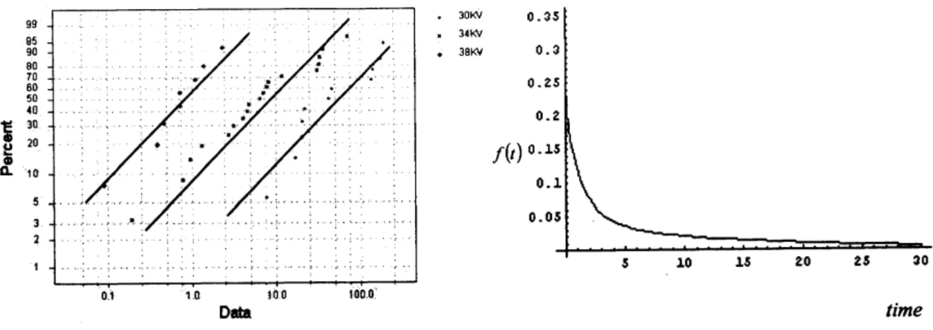
1 $30\mathrm{K}\mathrm{V}$ 7.74 17.05 20.46 21.02 22.66 43.40 47.30 139.07 144.12 175.88 194.90 0.19 0.78 0.96 1.31 2.78 3.16 4.15 4.67 4.85 6.50 7.35 2 $34\mathrm{K}\mathrm{V}$ 8.01 8.27 12.06 31.75 32.52 33.91 36.71 72.89 3 $38\mathrm{K}\mathrm{V}$ 0.09 0.39 0.47 0.73 0.74 1.13 1.40 2.38 Field data 0.47 0.96 1.13 4.15 8.01 12.06 20.46 31.75 43.4 139.07

Itis intended in the exampletoestimatethelifetime

distribution

ofthe fieldunits which is modeled bythemixed

proportional hazards model.Before estimatingthe parameters,the probability plot

can

be roughlyused to test the

fitness of the model to agiven set of data. The experimental data

are

plotted in Figure 1. The conditional

probability ofthelifetime given

acovariate

followsthe Weibull

distribution

with adifferentscale parameterand

asame

shape parameter ffom it’s baseline

distribution

becausethe

covariate

just changes the scaleparameter

in

the

case

ofthe Weibullbaseline hazardratein this model. Therefore, datashould be nearby three straight lines

and thestraight lines shouldbeparallel. Figure 1shows that theseconditions

are

nearlysatisfied in thisexample.

Using the proposedmethod,

we

have $\hat{\lambda}=5.89\cross 10^{-9},\hat{\beta}=0.9208$, $\eta\wedge=0.492$, $(\hat{p}_{1},\hat{p}_{2},\hat{p}_{3})=(0.27,0.53,0.2)$

.

Theprobabilitydensityfunction forthe exampleis graphed in Figure 2.

$\not\subset\epsilon\frac{\mathrm{o}}{\emptyset}$

Figure 1. Weibull probability plot Figure 2.Probability densityffinction

References

1. AnsellJ.I., Phillips M.J.,Practicalaspectsof modeling of repairable systems datausing proportional hazard

models. Reliability Engineering and System Safety,

199758: 165-171.

2.

EverittB.S.,HandDJ.,Finite mixturedistributions,

Chapman&Hall, 1981.

3. HiroseH.,Mixture model of thepowerlaw. IEEE TransactionsonReliability, 199746: 146-153.

4. Jaisingh L.R., Dey D.K., Griffith W.S., Properties of amultivariate survival distribution generated by

a

Weibull&inverse Gaussianmixture,IEEE Transactions

on

Reliability,

199342:618-622.

5. JiangR.,MurthyD.N.P.,Modeling failure-databy mixture of 2Weibulldistributions: agraphical approach,

IEEE Transactions

on

Reliability,

199544:477-488.

6. JiangS.,KececiogluD.,Graphical representation oftwo

mixed-Weibull

distributions,IEEETransactions

on

Reliability,

199241:241-247.

7. Jiang S., Kececioglu D., Maximum likelihood estimates ffom censored data, for mixed- Weibull

distributions.IEEETransactions

on

Reliability,

199241:248-255.

8. JozwiakI.J.,Anintroductionto the studiesofreliabilityofsystemsusing the weibullproportional hazards

model. Microelectronics andReliability,

199737:915-918.

9. KalbfleischJ.D.,PrenticeR.L., Thestatisticalanalysis

_offailure

timedata,John Wiley&Sons, 1980.

10. Kumar D., Klefsjo B., Proportional hazards model:

areview.

Reliability Engineering andSystem Safety,

199444:

177-188.

11.

LauT.S.,Mixture models

in

hazard rates

estimation.

Commun.Statist-TheoryMeth.,

199827:

1993

0.

12. Martorell S, Sanchez A, Serradell V., Age-dependentreliabilitymodel considering effects of

maintenan

ce

andworking conditions. ReliabilityEngineeringand SystemSafety, 199964:19-31.

13. McClean S., Estimation for the mixed exponential distribution using grouped follow-up data. Applied

Statistics, 198636:313.

14. McLachlan GJ., Basford K.E., Mixturemodels

,.

_Inference

and applications to clustering, Marcel Dekker,

1987.

15.

Nelson W.,Accelerated testing

,.

Statisticalmodels, testplansand data analyses, John Wiley&Sons,

1990.

16.

Peng Y., Dear K.B.G, Anonparametric mixture model for

cure

rate estimation, Biometrics,

200059:

237-243.

17. Solomon P.J., Effect of misspecification of regression model in the analysis of survival data. Biometrica,

198471:291-293.

18. SyJ.P.,TaylorJ.M.G,Estimation in aCox proportional hazards

cure

model, Biometrics,

200056:227-236.

19. TitteringtonD.M.,SmithA.F.M.,MarkovU.E.,Statistical analysis

_offinite

mixture distribution,JohnWiley

&Sons, 1990.