A Multi-GPU Implementation of a Parallel Solver for Incompressible Navier-Stokes Equations Discretized by Stabilized Finite Element Formulations (Numerical Analysis : New Developments for Elucidating Interdisciplinary Problems II)

A Multi‐GPU

_{Implementation}

of

a

Parallel

Solver for

Incompressible

Navier‐Stokes

_Equations

Discretized

_by

Stabilized Finite Element Formulations

HUYNH

_{Quang Huy Viet,}

SUITO

Hiroshi

Graduate

School of

Environmental and Life

_Science,

_Okayama

_University

E‐‐mail: _hqhviet\emptyset_okayama−u.ac._{jp, suito@okayama‐u.ac.jp}

1

Introduction

For

_{solving partial}

differential_equations

_problems

in

_{Computational}

Fluid

Dynamics

(CFD),

finite ele‐

ment methodsareconventional numerical methods thatare

_particularly

used because of their_accuracy.

In

_solving

the Navier‐Stokes

_(NS)

equations

using

finite element methods for simulation of_{incompress‐}

ible

flows,

some instabilitiesarise fromthe_presenceof advectionterms or the

high Reynolds

number.

Hughes

and

_Tezduyar

etal.

_[1,

_{2, 3,}

_4]

_proposed

stabilized finite element formulations for

incompressible

flows. Stabilizationin

_solving

Navier‐Stokesequations isachieved

_{by adding}

twostabilizationterms to the Galerkin formulations of the Navier‐Stokes equations. The first stabilizationtermis the streamline

upwind

/\mathrm{P}\mathrm{e}\mathrm{t}\mathrm{r}\mathrm{o}\mathrm{v}

‐Galerkin

_(SUPG)

term. The second stabilizationtermisthepressure

stabilizing/Petrov‐

Galerkin

_(PSPG)

term. This stabilizedfiniteelement method has been showntobeveryeffective for the simulationof_{incompressible}flows.

In_engineering

_{applications,}

when

_{computational}

conditions become

stiff,

NS solvers

_might

not con‐

verge tosolutions withinanallowed time limitation. Therefore_{it is necessary}to

_develop

fast andaccurate NS solvers

using

parallel processing techniques. Traditionally, parallel

NS solvers are

_developed

_using

supercomputersorPC clusters with

parallel programming platforms

suchas

OpenMP

andMPI.

_Recently,

because modern

_{graphics processing}

units

_(GPUs)

havemany processorsor_cores, GPU

_computing

has

been

_recognized

as a

_{powerful platform}

to achieve

_{high performance}

insimulation and

_modeling

inthe

CFD. GPU

_computing

istheuseof GPUsin associationwith theuseof CPUsto

speed

up

computations.

A

_desktop

machineor aworkstation witha

powerful

GPU inside canachieve

_{extremely high}

levels of

performance

for_computationand simulation. The_necessityexiststo

_{develop parallel}

NS solversonGPUs

forvarious

_{engineering applications.}

In arecent_report

_[5],

we

briefly

described our

implementation

of asolver based onthe GPBi‐CG

algorithm

for 3\mathrm{D}

unsteady

Navier‐Stokes equations discretized

by

the SUPG

_/

PSPG stabilized finite

elementformulation_usinga

_single

GPU.In this paper, we_reporta newmulti‐GPU

_{implementation}

of the solver and shows

_performance

results.

2

Stabilized

Finite Element Formulations

2.1

_{Governing Equations}

We consider the

_following

dimensionless form of the Navier‐Stokes_equationsina

spatial

domain

$\Omega$\subset \mathrm{R}^{3}

:

\displaystyle \frac{\partial u_{i}}{\partial t}+u_{j}\frac{\partial u_{i}}{\partial x_{j}}=-\frac{\partial p}{\partial x_{i}}+\frac{1}{Re}\frac{\partial}{\partial x_{j}}(\frac{\partial u_{i}}{\partial x_{j}}+\frac{\partial u_{j}}{\partial x_{i}})

in $\Omega$,

(1)

\displaystyle \frac{\partial u_{i}}{\partial x_{i}}=0

in $\Omega$.

(2)

Here,

we

_adopt

the summation conventionon

repeated

indices that have values _{1, 2,} and 3. The

x,y,z axesinthe Cartesian coordinatesystemare

designated

as_{x_{i}, i} = 1

,

2,

3. Here,u_{i} representsthe

componentof the

_velocity

vectorfield\mathrm{u}in the

i^{th} dimension,

pstands for the scalarpressure

field,

and

Re denotes the

_Reynolds

number.

Letus discretize the

spatial

domain $\Omega$

by

elements

_{$\Omega$^{e},}

e= 1

,2\ldots,n_{\mathrm{e}l}. Let

S_{\mathrm{u}},

\mathcal{V}_{\mathrm{u}} be the trial and

testfunctionspacesfor

velocity

and

S_{p}, \mathcal{V}_{p}

(\mathcal{V}_{p}=S_{p})

be trial andtest functionspacesforpressure. The stabilized finite element formulation of the_equations

_(1)-(2)

with the SUPG

_/

PSPG stabilizationterms

canbe

_expressed

asfollows

[1]:

Find\mathrm{u}\in S_{\mathrm{u}} and

_{p\in S_{p}}

such that\forall \mathrm{w}\in \mathcal{V}_{\mathrm{u}}and

_{\forall q\in \mathcal{V}_{p}}

:

数理解析研究所講究録

\displaystyle \int_{ $\Omega$}w_{i}(\frac{\partial u_{i}}{\partial t}+\overline{u}_{j}\frac{\partial u_{i}}{\partial x_{j}})d $\Omega$-\int_{ $\Omega$}\frac{\partial w_{i}}{\partial x_{i}}pd $\Omega$+\int_{ $\Omega$}\frac{1}{Re}\frac{\partial w_{i}}{\partial x_{j}}(\frac{\partial u_{i}}{\partial x_{j}}+\frac{\partial u_{j}}{\partial x_{i}})d $\Omega$

+\displaystyle \sum_{e=1}^{n_{\mathrm{e}1}}\int_{$\Omega$_{\mathrm{e}}} $\tau$\overline{u}_{k}\frac{\partial w_{i}}{\partial x_{k}}(\frac{\partial u_{i}}{\partial t}+\overline{u}_{j}\frac{\partial u_{i}}{\partial x_{j}}+\frac{\partial p}{\partial x_{i}})d $\Omega$=0

,

(3)

\displaystyle \int_{ $\Omega$}q\frac{\partial u_{i}}{\partial x_{i}}d $\Omega$+\sum_{\mathrm{e}=1}^{n_{\mathrm{e}1}}\int_{$\Omega$_{\mathrm{e}}} $\tau$\frac{\partial q}{\partial x_{i}}(\frac{\partial u_{i}}{\partial t}+\overline{u}_{j}\frac{\partial u_{i}}{\partial x_{j}}+\frac{\partial p}{\partial x_{i}})d $\Omega$=0

,

(4)

where $\tau$isthe SUPG

/

PSPG stabilization_parameter. The formulationtocalculate theparameter $\tau$

is

_given

indetailsinthepaper

[1].

3

GPBi‐CG

_Algorithm

Algorithm

1 The

_{Unpreconditioned}

GPBi‐CG

x_{0} isaninitialguess,

r_{0}=b-Ax_{o}

;

Set

_{r_{0}^{*}=r_{0},}

_{t_{-1}=w_{-1}=0,}

_{$\beta$_{-1}=0}

;

forn=0,1, until

||r_{n}||\leq $\epsilon$||b||

do

p_{n}=r_{n}+$\beta$_{n-1}(p_{n-1}-u_{n-1})

,

$\alpha$_{n}=\displaystyle \frac{(r_{\dot{\mathrm{o}}},r_{n})}{(r_{\mathrm{o}}^{*},Ap_{n})},

y_{n}=t_{n-1}-r_{n}-$\alpha$_{n}w_{n-1}+$\alpha$_{n}Ap_{n},

t_{n}=r_{n}-$\alpha$_{n}Ap_{n},

$\zeta$_{n}=\displaystyle \frac{(y_{n},' y_{n})(At_{n},t_{n})-(y_{n},t_{n})(At_{n},y_{n})}{(At_{n}At_{n})(y_{n},y_{n})-(y_{n},At_{n})(At_{n},y_{n})},

$\eta$_{n}=\displaystyle \frac{(At_{n},' At_{n})(y_{n},' t_{n})-(y_{n},At_{n})(At_{n},t_{\mathfrak{n}})}{(At_{n}At_{n})(y_{n}y_{n})-(y_{n},At_{n})(At_{n},y_{n})},

(if

n=0, then

$\zeta$_{n}=\displaystyle \frac{(At_{n},t_{n})}{(At_{n},At_{n})},

$\eta$_{n}=0

),

\mathrm{u}_{n}=$\zeta$_{n}Ap_{n}+$\eta$_{n}(t_{n-1}-r_{n}+$\beta$_{n-1}u_{n-1})

,

z_{n}=$\zeta$_{n}r_{n}+$\eta$_{n}z_{n-1}-$\alpha$_{n}u_{n},

x_{n+1}=x_{n}+ $\alpha$ p_{n}+z_{n},

r_{n+1}=t_{n}-$\eta$_{n}y_{n}-$\zeta$_{n}At_{n},

$\beta$_{n}=\displaystyle \frac{$\alpha$_{n}}{$\zeta$_{n}}\frac{(r_{0}^{*},r_{n+1})}{(r_{\dot{0}},r_{n})},

w_{n}=At_{n}+$\beta$_{n}Ap_{n}

; end for

stabilized finite element method leadstoa

large

and

This linear

_equation

_systemis solved

_{by using}

the

To

implement

the GPBi‐CG

_algorithm

onthe GPU

platform,

weused the Nvidia’s GPU linear

_algebra

libraries cuSPARSE

_[7]

and cuBLAS

_[8]

to

_implement

four basic vector _operationsof the

_algorithm:

SpMV, DOT,

AXPY and SCALasdescribed below.

\bullet

\mathrm{S}\mathrm{p}\mathrm{M}\mathrm{V}

:the sparse matrix‐vector

_product,

. DOT: the inner

_product,

\bullet AXPY: adda

_multiple

ofonevector to

_another,

\bullet SCAL:

_scaling

avector

by

aconstant.

The

_{SpMV operation}

is

_{implemented by using}

thecuSPARSE

_library.

The

_DOT,

AXPY and SCAL

operationsare

_{implemented by using}

thecuBLAS

_library.

4

Multi‐GPU

_{Implementation}

To extendto multi‐GPU _{implementation} of theGPBi‐CG

algorithm,

we implemented themulti‐GPU

versionof

SpMV,

DOT,

AXPY,

andSCAL_operations

_by

_usingthe MPI

library,

thecuSPARSE

library

and the cuBLAS

_library.

It is trivialto

_implement

themulti‐GPU version of the DOT,

AXPY,

and

SCAL_{operations by using} the MPI

library

andcuBLAS

_library.

_However, the_{implementation} ofthe

multi‐GPUversion of the

SpMV

operationisnot

_{straightforward.}

It is carriedout

_{by subdividing}

the

computationaldomain into subdomains thataredistributedovertheGPUsby usingthe MPI

library.

To

reduce communicationcost,we

develop

anefficient_procedurethat eachGPUreceives from other GPUs

only

data eachGPUneeds. We consider the_problemof matrix‐vector_{multiplication}ofa_{sparse matrix}

Aandadensevector b. Wepartitionthe matrix Ainto groups ofadjacent completerowsand assign

onesuch grouptooneGPU. EachGPUis now

obligated

to_computeentriesof the resultvectorAbthat match with the_partitioned rowsof the matrixAto formapartialresultof the resultvectorAb. This

submatrix‐vectorcomputationcanbe carriedoutaftereachGPUreceivesthe entries of thevectorb that

correspondtonon‐zeroentries intherowsof the submatrixAwhichare

_assigned

toeachGPU. Asimple

implementation

forthisproblemisto

_implement

acode that all the GPUsreceivesall the entries of the

entirevectorb. However,thisimplementationisnotefficientbecause the number ofnon‐zeroentries per

a rowofa_sparsematrix

_{generated by}

fimite elementmethodsis small. To solve this

problem,

we

develop

an efficient_procedurethat each GPU receives from other GPUs

only

the entries of the vector b which eachGPUneedsto_computesubmatrix‐vector

_{multiplications.}

5

Performance Results

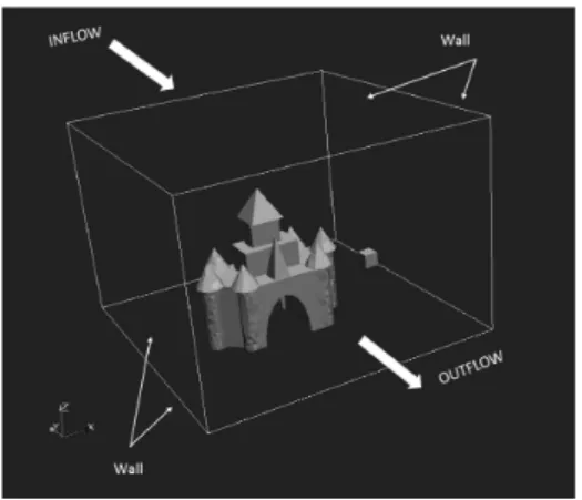
Figure 1: _{Computational}domain of the testproblem

We consideratestproblemwhichconsistsofan

object

immersed inafluid domainasshownin

_Fig.

1.

Starting

fromasurfacemesh,wecreatedthreetetrahedral mesheswith differentresolutions. We carried

outthe_{computationby using}aGPU_systemwith the

following

_{specification:}

\bullet _{Intel XeonCPUE5630,}2.

_{53\mathrm{G}\mathrm{H}\mathrm{z},}

\bullet 2GPUs‐Tesla

_C2070,

\bullet 24GB

System Memory.

Thble 1: _Speed‐upratiosandexecution times

We measured thetimeof theexecutionontwoGPU devices and thatoftwoCPU threads. As shown inTab. 1,theGPUexecution is1.8 timesfaster than the CPUexecutionfor the

large

mesh with 638447 elements. The

speedup

ratioincreasesas_{the number of elements of meshes increases.}

6

Conclusions

Weproposeanefficient

_{implementation}

ofamulti‐GPU

parallel

solver basedontheGPBi‐CG

algorithm

for 3\mathrm{D}

_unsteady

Navier‐Stokesequationsdiscretized

_by

the stabilized finite element formulations. We

develop

a

hybrid

CPU‐GPU_strategythat distributes the

_computation

acrossGPUs

_{by using}

the MPI

library.

In futureresearch,we

plan

toevaluate the

_scalability

of the_program

_(speedup

factorversusthe

number of GPU

_devices)

inmulti‐GPU

_{high‐performance computing}

systems. We also

_plan

to

_improve

thecurrent

_{implementation by using multigrid‐ preconditioners.}

Acknowledgment

This workwas

_{supported by Japan}

Science and

_{Technology Agency,}

Core Research for Evolutional Science

and

_Technology

_{(JST‐CREST).}

The first author would liketo

_acknowledge

Mr.

Ryota

Yamane

_(Okayama

University)

for

_providing

the STL file used fortest _{computations.}

References

[1]

T. E.

_Tezduyar,

Stabilized fimite element formulations for

_{incompressible}

flowcomputations,Advances

in

_Applied

Mechanics28

₍₁₉₉₂₎

1‐44.

[2]

T. E.

_Tezduyar,

S.

_Mittal,

S. E.

_Ray,

R.

_{Shih, Incompressible}

flow _computationswith stabilized bilinear and linear

_equal

order

_{interpolation velocity}

pressure

elements, Computer

Methodsin

Applied

Mechanics and

_Engineering

95

₍₁₉₉₂₎

221‐242.

[3]

$\Gamma$.

Shakib,

T. J. R.

Hughes,

Z.

Johan,

A new finite element formulation for

computational

fluid

dynamics:

X. the

compressible

Euler and Navier‐Stokes_equations,

_Computer

Methodsin

_Applied

lMechanics

and

_Engineering

89

₍₁₉₉₁₎

141‐219.

[4]

L. P.

Franca,

S. L.

_Fhey,

T. J. R.

_Hughes,

Stabilized finite element methods: I.

_application

tothe advective‐diffusive

_{model, Computer}

Methodsin

_Applied

Mechanics and

Engineering

95

₍₁₉₉₂₎

235‐ 276.

[5]

V.

_Huynh,

H.

_Suito,

A GPU Parallel Solver for 3D

_{Incompressible}

Navier‐Stokes

_Equations

Dis‐

cretized

_by

the SUPG

_/

PSPG Stabilized Finite Element

_Formulation,

GPU

_Technology

Confer‐ ence _{2016, http://\mathrm{o}\mathrm{n}}‐demand._gputechconf.

$\Gamma$ 1\mathrm{u}\mathrm{i}\mathrm{d}_{-}_Dynamic\mathrm{s}_{-}\mathrm{C} $\Gamma$ \mathrm{D}_{-}01_{-}\mathrm{P}6160_{-}\mathrm{W}\mathrm{E}\mathrm{B}.pdf

(Accessed

Oct.

2016).

[6]

S. L.

_Zhang,

GPBi‐CG: Generalized

product‐type

methods basedonUi‐CG for

solving nonsymmetric

linearsystems,SIAM J. Sci.

Comput.

18

₍₁₉₉₇₎

537‐551.

[7]

CuSPARSE,

https:

//developer.

nvidia.

_com/cusparse

_(accessed

Oct.

_2016).

[8]

CuBLAS,

https:

//developer.

nvidia.com/cublas

_(Accessed

Oct.

_2016).