Dissipative Schemes for the Ginzburg-Landau Equations (Recent Developments of Numerical Analysis and Numerical Computation Algorithms)

Dissipative

Schemes for the Ginzburg-Landau Equations

Takayasu

Matsuo and

Eitaro Torii

1

Abstract

Twoexisting and

one

new Galerkin schemes for the Time-Dependent

Ginzburg-Landau (TDGL) equations

are

presented. The schemes have

an

welcome feature

in common that each keeps a discrete counterpart of the original energy

dissipa-tion property of the TDGL. Based on the Lyapunov theory, asymptotic behavior

of the solutions ofthe schemes are discussed, whichis then confirmed by numerical

experiments.

1

Introduction

The phenomelogical behavior ofsuperconductivity is governed by the so-called

Ginzburg-Landau model. The model in the so-called “zero electric potential gauge” is described

as

the following time-dependent Ginzburg-Landau (TDGL) equations:

$\eta\frac{\partial\psi}{\partial t}+\frac{1}{2}\{(\frac{i}{\kappa}\nabla+A)^{2}\psi+(|\psi|^{2}-1)\psi\}=0$ in $\Omega$, (la)

$\frac{\partial A}{\partial t}+{\rm Re}[\overline{\psi}(\frac{i}{\kappa}\nabla+A)\psi]+\nabla\cross(\nabla\cross A-H)=0$ $i_{l1}\Omega$, (lb)

where $\Omega\subset \mathbb{R}^{d}$ is

a

bounded subdomain with smooth boundary, _$\kappa>0$

is the material

constant called the Ginzburg-Landau parameter, $\eta>0$ is the friction coefficient, $H\in \mathbb{R}^{d}$

is the applied magnetic field, $\psi$ : $\Omega\cross[0, T]arrow \mathbb{C}$ is the complex-valued order parameter

which denotes the conducting state of the material, and $A$ : $\Omega\cross[0, T]arrow \mathbb{R}^{d}$ is the

magnetic potential. By $\overline{\psi}$

we

mean

the complex conjugate

of

$\psi$

.

The associated boundary

conditions

are:

$\nabla\psi\cdot n=0$, $A\cdot n=0$_, $n\cross(\nabla\cross A-H)=0$

on

$\partial\Omega$. (lc)

where $n$ is the exterior unit normal of the boundary $\partial\Omega$. For this gauge choice and the

well-posedness of the associated Cauchy problem,

see

[2].

The advantage of this particular gauge choice is that the problem

can

be viewed

as

a

gradient-flow of the Ginzburg-Landau energy functional:

$E( \psi, A)=\int_{\Omega}\{\frac{1}{2}|(\frac{i}{\kappa}\nabla+A)\psi|^{2}+\frac{1}{4}(1-|\psi|^{2})^{2}+\frac{1}{2}|\nabla\cross A-H|^{2}\}dx$, (2)

$\eta\frac{\partial\psi}{\partial t}=-\frac{\overline{\delta}E}{\delta\overline{\psi}}$, $\frac{\partial A}{\partial t}=-\frac{\delta E}{\delta A}$, (3)

lGraduate School of Information Science and Technology, The University of Tokyo, Hongo 7-3-1,

where $\delta E/\delta\overline{\psi}$and $\delta E/\delta A$denote variationalderivatives. This energyin otherwords

serves

as a

Lyapunov functional ofthesystem, and this suggests

us

to employnumerical schemes

having

some

discrete counterpart of this property

for

stability and correct asymptotic

behavior. So far several fully-implicit schemes having discrete Lyapunov functional have

been proposed [3, 10], but due to their nonlinearity

some

iterative solver was necessarily

required, andthus they were relatively expensive. A remedy to overcome this difficulty is

to introduce

some

linearization technique, such as the one proposed in [9], which enables

us

to design a linearly-implicit scheme that still keeps discrete dissipation property in

some

sense.

As

its price, however, theresulting scheme

can

be unstable, since the discrete

energy function in this

case

does not necessarily

serve

as Lyapunov functional.

In the present paper, after briefly reviewing the existing fully-implicit schemes [3, 10],

we

present

a

linearly-implicit scheme with the linearization technique [9]. Then the

qual-itative behavior of discrete solutions for each scheme is discussed based

on

the Lyapunov theory. In order to simplify the discussion, in what follows

we

limit ourselves to the

simplified model ignoring all the magnetic effects:

$\eta\frac{\partial\psi}{\partial t}=\frac{1}{2}\{\frac{\triangle\psi}{\kappa^{2}}+(1-|\psi|^{2})\psi\}$ in $\Omega$, _{$\nabla\psi\cdot n=0$}

on

$\partial\Omega$. (4)

This still deserves investigation since it still keeps interesting physical solutions such

as

vortices, and

a

Lyapunov functional:

$E( \psi)=\int_{\Omega}\{\frac{1}{2}|\frac{\nabla\psi}{\kappa}|^{2}+\frac{1}{4}(1-|\psi|^{2})^{2}\}dx$. (5)

The simplified equation (4) is formally agradient flow with respect to the energy:

$\eta\frac{\partial\psi}{\partial t}=-\frac{\delta E}{\delta\overline{\psi}}$. (6)

Wealso

assume

$d=2$_for brevity (we consider, say, aunit disk). Let $H_{c}^{1}(\Omega)$ be thestandard

Sobolev space ofcomplex-valuedfunctions and $(\cdot,$ $\cdot)$ be itsassociated inner product. Let $S_{d}$

and $W_{d}$ be thefinite-dimensionalsubspaces in $H_{c}^{1}(\Omega)$ for trial and test functions satisfying

$S_{d}\subseteq W_{d}$ (in most

cases we

simplytake _{$S_{d}=W_{d}$}, in particular to the standard piecewise

linear function space).

2

Fully-implicit Schemes for the simplified

GL

equa-tion

Amethod for designing Galerkinschemes preserving energydissipation property hasbeen

proposed in [8]. By applying the method, we reach the following fully-implicit scheme

as

Scheme 1 (Fully-implicitscheme 1 [10]). Suppose

an

initial data$\psi^{(0)}\in S_{d}$ is given. Find

$\psi^{(m)}\in S_{d}(m=1,2, \ldots)$ such that

for

any $\phi\in W_{d}$

$\eta(\frac{\psi^{(m+1)}-\psi^{(m)}}{\Delta t},$ $\phi)=-(\frac{\partial E_{d}}{\partial(\nabla\overline{\psi}^{(m+1)},\nabla\overline{\psi}^{(m)})},$$\nabla\phi)-(\frac{\partial E_{d}}{\partial(\overline{\psi}^{(m+1)},\overline{\psi}^{(m)})},$$\phi)$ , where

$\frac{\partial E_{d}}{\partial(\nabla\overline{\psi}^{(m+1)},\nabla\overline{\psi}^{(m)})}$ $=$ $\frac{1}{2\kappa^{2}}(\frac{\nabla\psi^{(m+1)}+\nabla\psi^{(m)}}{2})$,

$\frac{\partial E_{d}}{\partial(\overline{\psi}^{(m+1)},\overline{\psi}^{(m)})}$ $=$ $- \frac{1}{2}(1-\frac{|\psi^{(m+1)}|^{2}+|\psi^{(m)}|^{2}}{2})(\frac{\psi^{(m+1)}+\psi^{(m)}}{2})$ .

This scheme has

a

desired dissipation property.

Proposition 1 (Dissipation property

of Scheme 1

[10]).

Let

$\psi^{(m)}(m=1,2, \ldots)$ be

the

solutions

_of

Scheme

1. Then thefollowing discrete dissipationproperty holds:

$\frac{1}{\triangle t}\int_{\Omega}E(\psi^{(m+1)})-E(\psi^{(m)})dx=-2\eta\int_{\Omega}|\frac{\psi^{(m+1)}-\psi^{(m)}}{\triangle t}|^{2}dx\leq 0$.

That is, in

Scheme

1 the original

energy

$E$ dissipates

as

in the continuous

case.

This

implies that the asymptotic behavior of the approximate solutions must be quite similar

to that ofthe originalTDGL (strictlyspeaking, tothat ofthe corresponding ODE derived

by discretizing the space variable).

In [3],

an

implicit Euler type scheme is derived from the

energy functional

based

on

minimization

theory.

Here

onlythe resulting

scheme

is shown.

Scheme 2 (Fully-implicit scheme 2 [3]). Suppose

an

initial data $\psi^{(0)}\in S_{d}$ is given. Find

$\psi^{(m)}\in S_{d}(m=1,2, \ldots)$ such that

for

any $\phi\in W_{d}$

$\eta(\frac{\psi^{(m+1)}-\psi^{(m)}}{\triangle t},$$\phi)=-\frac{1}{2\kappa^{2}}(\nabla\psi^{(m+1)}, \nabla\phi)-\frac{1}{2}((|\psi^{(m+1)}|^{2}-1)\psi^{(m+1)}, \phi)$ .

Proposition 2 (Dissipation property

of

Scheme 2

[3]).

Let

$\psi^{(m)}(m=1,2, \ldots)$ be the

solutions

_of

Scheme 2. Then the following discrete dissipation property holds:

$\frac{1}{\triangle t}\int_{\Omega}E(\psi^{(m+1)})-E(\psi^{(m)})dx\leq-2\eta\int_{\Omega}|\frac{\psi^{(m+1)}-\psi^{(m)}}{\triangle t}|^{2}dx\leq 0$ .

Thus the scheme should have similar asymptotic behavior

as

above; in fact, in [3],

a

detailed discussion

on

the asymptotic behavior is given for the full TDGL (1).

In these two silnilar schelnes, however, we find several cssential differences. First,

notice that the first equality in Prop. 1 is replaced with an inequality in Prop. 2, whose

equalitydoesnotholdsin general (this

can

be understood by carefully inspectingits proof;

interested readers may refer to [3]$)$

.

Since

in the continuous case, the equality holds: $( d/dt)\int Edx=-2\eta\int|\psi_{t}|^{2}dx$,

we can

say that

Scheme

1 is closer to the original

TDGL.

Although the implicit Euler

scheme

happily keeps the Lyapunovfunctional, thedissipation

(how

the energy

is dissipated) is slightly stronger

there than

it

should be.

Second,

Scheme 1

should be second order with respect to $\triangle t$ due to its temporal symmetry, while Scheme 2

is only first order.

Both schemes have

an

unwelcome feature in

common:

they

are

fully-implicit, and

necessarily require time-consuming iterative solver. This disadvantage becomes

even

more

crucial, if

we

consider the full TDGL,

or

like to proceed to the $d=3$

cases.

In the next

section,

we

consider

a

linearly-implicit scheme in order to

overcome

this disadvantage.

3

A Linearly-Implicit

Scheme

for the simplified

GL

equation

By combining the method [8] and the linearization technique [9],

we

can

derive the

follow-ing linearly-implicit scheme.

Scheme 3 (Linearly-implicit scheme). Suppose an initial data $\psi^{(0)}\in S_{d}$ and a starting

value $\psi^{(1)}$

are

given. Find $\psi^{(m)}\in S_{d}(m=2,3, \ldots)$ such that

for

any $\phi\in W_{d}$

$\eta(\frac{\psi^{(m+1)}-\psi^{(m-1)}}{2\triangle t},$$\phi)=-(\frac{\partial E_{d}}{\partial(\nabla\overline{\psi}^{(m+1)},\nabla\overline{\psi}^{(m)},\nabla\overline{\psi}^{(m-1)})},$ $\nabla\phi)-(\frac{\partial E_{d}}{\partial(\overline{\psi}^{(m+1)},\overline{\psi}^{(m)},\overline{\psi}^{(m-1)})},$$\phi)$

where

$\frac{\partial E_{d}}{\partial(\nabla\overline{\psi}^{(m+1)},\nabla\overline{\psi}^{(m)},\nabla\overline{\psi}^{(m-1)})}$ $=$ $\frac{1}{2\kappa^{2}}\{b\nabla\psi^{(m)}+(1-b)\frac{\nabla\psi^{(m+1)}+\nabla\psi^{(m-1)}}{2}\}$ ,

$\frac{\partial E_{d}}{\partial(\overline{\psi}^{(m+1)}.\overline{\psi}^{(m)},\overline{\psi}^{(m-1)})}$ $=$

$\frac{a}{2}(-1+\frac{\psi^{(m+1)}+\psi^{(m-1)}}{2}\overline{\psi}^{(m)})\psi^{(m)}$

$+ \frac{1-a}{2}(-1+|\psi^{(m)}|^{2})(\frac{\psi^{(m+1)}+\psi^{(m-1)}}{2})$ ,

and $a,$$b\in \mathbb{R}$

are

scheme parameters.

The scheme parameters $a,$$b$ should be chosen carefully, since they severely affect the

stability of the resulting scheme as will be shown below. Observe that the scheme is

linear withrespect to thelatest value$\psi^{(m+1)}$

.

This schemeenjoys the following dissipation

property.

Theorem 1 (Dissipation property of Scheme 3). Let $\psi^{(m)}(m=2,3, \ldots)$ be the solutions

of

Scheme 1. Then the following discrete dissipation property holds:

where

$E_{d}(\psi^{(m+1)}, \psi^{(m)})$

$=$ $\frac{1}{4}\{a(1-\psi^{(m+1)}\overline{\psi}^{(m)})(1-\overline{\psi}^{(m+1)}\psi^{(m)})+(1-a)(1-|\psi^{(m+1)}|^{2})(1-|\psi^{(m)}|^{2})\}$

$+ \frac{1}{2\kappa^{2}}\{b(\frac{\nabla\psi^{(m)}\cdot\nabla\overline{\psi}^{(m+1)}+\nabla\overline{\psi}^{(m)}\cdot\nabla\psi^{(m)}}{2}I+(1-b)(\frac{|\nabla\psi^{(m+1)}|^{2}+|\nabla\psi^{(m)}|^{2}}{2})\}\cdot$

(7)

Note that

now

the discrete energy function (7) depends

on

two consecutive numerical

solutions (i.e. it is “multistep”), and quadratic with respect to the latest value $\psi^{(m+1)}$;

this is the key for the linearization. The scheme parameters $a,$$b$ appear as thecoefficients

of the linear combination of the quadratic approximations. The theorem states that for

any

choice of $a,$$b$, the

discrete

dissipation property

holds

in the

above

sense.

The

dis-crete energy function (7) is, however, totally different from the original one (5), and as

a

consequence the discrete dissipation property does not immediately imply the correct

asymptotic behavior,

as

was

the

case

in the fully-implicit schemes.

Still, thediscreteenergy functiongives

us

useful information for designinggood (stable)

schemes;

more

specifically, for the choice ofappropriate scheme parameters $a,$$b$. Below

we

demonstrate this. The first step is to rewrite the energy function

as

follows.

$E_{d}(\psi^{(m+1)}, \psi^{(m)})$ $=$ $\frac{1}{4}\{|1-\psi^{(m+1)}\overline{\psi}^{(m)}|^{2}+(0-1)|\psi^{(m+1)}-\psi^{(m)}|^{2}\}$

$\frac{1}{2\kappa^{2}}\{|\frac{\nabla\psi^{(m+1)}+\nabla\psi^{(m)}}{2}|^{2}+(1-2b)|\frac{\nabla\psi^{(m+1)}-\nabla\psi^{(m)}}{2}|^{2}\}.(8)$

Let

us

then consider

a

“doubled” phase space $(\psi^{(m+1)}.\psi^{(m)})$, and regard that Scheme

3

defines a discrete map on the doubled space: $(\psi^{(m-1)}, \psi^{(m-2)})\mapsto(\psi^{(m+1)}, \psi^{(m)})$. We then

observe that depending

on

the parameters $a,$$b$ the dynamical system

can

behave in the

following three ways.

1. When $a<1$

or

$b>1/2,$ $E_{d}(\psi^{(m+1)}, \psi^{(m)})$ obviously is not bounded from below, and

thus it can

never

serve as Lyapunovfunctional. In this case, bylosing the Lyapunov

property the system can be unstable.

2. When $a=1$ and $b=1/2$, which here

we

call the “critical” case, the

energy

function

is bounded and

can serve as

Lyapunov

functional.

By the Lyapunov theory, the

dynamical systemit governsasymptoticallytends to the minimizers. Butby

a

careful

glance we notice that the dynamics is a bit different from the original one. Let us

consider the global minimizers $\int F_{d}\lrcorner(\psi^{(m+1)}, \psi^{(m)})dx=0$. In viewof(8),

we see

that

theglobal minimizers

are

such points that $\psi^{(m+1)}\overline{\psi}^{(m)}=1$ and _{$\nabla(\psi^{(m+1)}+\psi^{(m)})=0$}.

This allows

an

oscillatory (steady state” solution $\psi^{(m)}=c,$ $\psi^{(m+1)}=1/\overline{c}$ where

$c\in \mathbb{C}$ is

an

arbitrary constant. This is in fact “steady state” in that in the doubled

original

undoubled space,

however, it represents

an

oscillatory

solution

$carrow 1/\overline{c}arrow$

$carrow 1/\overline{c}arrow\cdots$. Thus

we

conclude that in the critical case, the system is equipped

with aLyapunov functional, but the dynamics isdifferent such that it allows spurious

fixed points (in the doubled space).

3. When $a>1$ and $b\leq 1/2$, the spurious fixed points vanish, and the Lyapunov

functional allows only original steady state solutions as its fixed points.

In the last case, the dynamical system is expected to behave the

same

way

as

the

fully-implicit cases, although the corresponding linearly-implicit scheme is far cheaper.

We like to generalize the above observation

as

follows: as an unavoidable consequence of

the linearization, theresulting scheme should be necessarily multistep, and the associated

dynamical system should be understood in the

doubled

(or

more

higher) phase space.

There are often degrees of freedom in the definition of multistep energy functions, and it

crucially determines the dynamics, which is then observed as its (numerical) stability. In

some

happy cases, such as the above, by carefully choosing the free (scheme) parameters

we can enforce the scheme (the dynamical system) to behave the same as the original

system. A question, however, _{still remains that} in which circumstances we can find such

“happy”

cases.

Inparticular, whether

or

not

we

can

do that for any PDEs is

an

important

open problem to be answered.

4

Numerical Examples

In this section wepresent numericalexamples thatillustratethe discussionin theprevious

section. We here test Scheme 3, with two parameter sets $(a.b)=(0.9,0.5)$ and $(2. -0.5)$,

each ofwhich corresponds to the first and third patterns described above. For comparison,

we also test the standard semi-implicit scheme, where the diffusion term is discretized in

time by the implicit Euler, and the nonlinear term by the explicit Euler. Weset theTDGL

parameters to be $\eta=1,$ $\kappa=15$, and solved the simplified TDGL

on

the unit disk with a

triangulation of 9,375 elements by FreeFEM. As the initial data,

we

set the two vortices

ofindices $+1$ and $-1$. With this setting, it is known that the annihilation (disappearing

by merging) ofvortices should

occur.

First we show a result with a fine time mesh $\triangle t=0.1$. We tested the semi-implicit

scheme and Scheme 3 with $(a, b)=(2, -0.5)$. and found no difference; both schemes run

quite happily inthis

case.

We show the result in Fig. 1.

The corresponding energy profiles are shown in Fig. 2. For Scheme 3, we calculated

$E_{d}$ (the multistep energy function (7)) and $E$ (the original energy function (5)). For the

semi-implicit scheme,

we

calculated only the latter. Inthis setting, all the three lines well

agree.

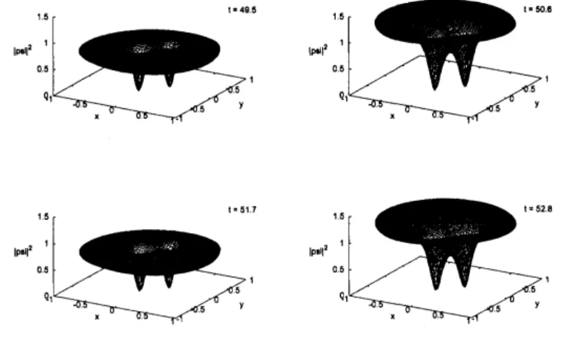
The semi-implicit scheme, however, becomes unst able as$\triangle t$ increases. We demonstrate

itby setting$\triangle t=1.1$in Fig. 3; theyarethe snapshots offourconsecutivetimestepsaround

$t\cdot 0D$ $t\cdot un$ $\iota\cdot 473$

t.n2 $s\iota$ ,.$1\infty D$

Figure 1: Evolution of the solution with $\triangle t=0.1$: the semi-implicit scheme and Scheme 3

with $(a.b)=(2, -0.5)$

$\omega\subset\frac{O\lambda}{\omega})$

$0$ 20 4) 60 80 100

time

Figure 2: Evolution of the energies with $\triangle t=0.1$: the semi-implicit scheme and Scheme

3

out with the

same

coarse

time step

as

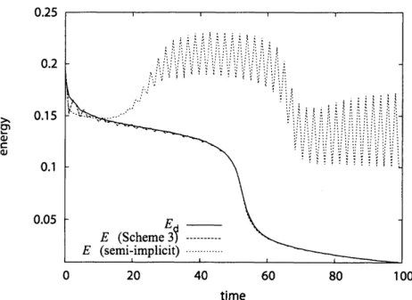
shown in Fig. 4. The

energy

profiles

are

shown in

Fig. 5, where

we

can

observe oscillation in the semi-implicit scheme.

Figure 3: Evolution of the solution with $\triangle t=1.1$: thesemi-implicit scheme

$t=0D$ $t=ua$ $t\cdot 473$

$t=517$ $t=55D$ $t=\infty 9$

Figure 4: Evolution of the solution with $\triangle t=1.1$: Scheme

3

Finally

we

test Scheme 3 with the parameters $(a, b)=(0,9,0.5)$ with $\triangle t=0.5$

.

As

shownin Fig. 6, theresult is catastrophic. This agrees withthe discussion in the previous section.

5

Concluding

Remarks

In this paper,

we

presented

a

new

linearly-implicit dissipativescheme for thetime-dependent Ginzburg-Landau (TDGL) equations without magnetic effects. and discussed its

asymp-$\mathring{\omega\subset\frac{\lambda}{\Phi}})$

$0$ 20 40 60 80 100

time

Figure 5: Evolution of the energies with$\triangle t=1.1$: the semi-implicit scheme and Scheme 3

with $(a.b)=(2, -0.5)$

$t\cdot 0$ $t\cdot u$ $\iota\cdot us$

$\iota\cdot \mathcal{B}$ $t\cdot 32s$ _ts41

$|\mu\cup^{\wedge}2$

totic behavior from the perspective of the Lyapunov theory. Two existing fully-implicit

schemes

were

also shown and discussed.

It is possible to construct linearly-implicit dissipative scheme for the full

TDGL

(with

magnetic effects) based on the same idea employed in this paper. That will be reported

elsewhere

soon.

Ackowledgements

This work

was

supported by a Grant-in-Aid for Encouragement of Young Scientists (B)

of the Japan Society for the Promotion ofScience.

References

[1] Arnold, D. N., Bochev, P. B., Lehoucq, R. B., Nicolaides, R. A., and Shashkov, M.

(eds.), Compatible Spatial Discretizations, Springer, New York, 2006.

[2] Du, Q., Global Existence and Uniqueness of Solutions of the Time-Dependent

Ginzburg-Landau Model for Superconductivity, Appl. Anal., 53 (1994),

1-17.

[3] Du, Q., Finite Element Methods for the Time-Dependent Ginzburg-Landau Model

ofSuperconductivity, Comput. Math. Appl., 27 (1994), 119-133.

[4] Furihata, D., Finite Difference Schemes for $\frac{\partial u}{\partial t}=(\frac{\partial}{\partial x})^{\alpha}\frac{\overline{6}G}{\delta v}$ That Inherit Energy

Con-servation

or

Dissipation Property, J. Comput. Phys., 156 (1999),

181-205.

[5] Furihata, D. and Matsuo, T., A Stable, Convergent, Conservative and Linear Finite

Difference Scheme for the Cahn-Hilliard Equation, Japan J. Indust. Appl. Math., 20

(2003), 65-85.

[6] Hairer, E., Lubich, C., and Wanner, G., Geometric Numerical Integration, Springer,

Heidelberg, 2006.

[7] Leimkuhler, B. and Reich, S., Simulating Hamiltonian Dynamics, Cambridge,

Cam-bridge, 2004.

[8] Matsuo, T., Dissipative/ConservativeGalerkin MethodUsingDiscretePartial

Deriva-tivefor Nonlinear EvolutionEquations, J. Comput. Appl. Math., 218 (2008),

506-521.

[9] Matsuo, T. and Furihata, D., Dissipative or Conservative Finite-Difference Schemes

for Complex-Valued Nonlinear Partial Differential Equations, J. Comput. Phys.,

171

(2001), 425-447.

[10] Mori, S., Numreical Schemes Perserving the Dissipation Property of the

Ginzburg-Landau Equations (in Japanese), masters thesis, the Universityof Tokyo,

2008.

[11] F.-Pell\’e, J., Kaper, H. G.. and Tak\’a\v{c}, P., Dynamics of the Ginzburg-Landau