Issues on the Optimal Financial Policy and Incentive in a Firm(Mathematical Models and Decision Making under Uncertainty)

Issues

on

the

Optimal

Financial

Policy

and

Incentive in

a

Firm

Kiyoyuki Horikawa (堀川 清之)

Graduate School of Economics,

Osaka University

(大阪大学大学院 経済学研究科)

1

Introduction

Modigliani and Miller (1958) [6] established the financial policy ofafirm that if there

are

no tax and transaction cost, the value of a firm is independent to the firm’s liabilities.

After this seminalinvestigation,many triedtorelaxitsconditions. They are, for example,

the debt affection to a firm’s taxable capital, the bankruptcy cost, and the agency costs.

In these ways, a firm’s manager determines optimal liabilities taking into account its

benefit and cost.

In addition to their studies, we in this paper $\mathrm{i}\mathrm{n}\mathrm{t}\mathrm{r}\mathrm{o}\mathrm{d}_{11}\mathrm{c}\mathrm{e}$the incentive effect by firm’s

financial policy from both shareholders and managers. Let $11\mathrm{S}$ imagine

a

venturecompany.

For its small shareholders’ equity,

some

additional liabilities bring it the great leverage

effect. In addition, that leverage effect also brings the great incentive for itsmanager to

make effort. On the contrary, that might be weakfor

a

giant company because relatively,

the leverage effect is weak for the large shareholders’ equity. Let us also consider the

case

to increase their capital: toissue corporate bond or share. Generallyspeaking, that

self-financingof a venture

seems

the way to provide its employees from its growth. However

is the opposite $\mathrm{t}\mathrm{r}11\mathrm{e}^{7}$ That is; the possibility ofits growth brings incentive ofemployees.

Morellec and Smith Jr. (2004) [7] have introduced that incentive effect only from the view

of shareholders. Cadenilias et al. (2004) [2] have focused

on

the relationship not only the

shareholders but also the manager. Howevertheir work of the managers’ utility does not

consider thesize of firm; asmy previous example, it is

a

venture firm

or

agiant company.

As we have described above, financial policy in ventures and giant companies might be

quite different. We examineto depict it more clearly at Section 2.2 and 2.3.

We illustrate the problem

as

follows: a risk averse manager receives

some

levered

shares

as

his compensation. This is the only

source

of his compensation. For a certain

liabilities and compensation level, he decidesacertainlevel of his effort and project, which

is expressed by volatility, to maximize his final utility. His effort requires cost, however

his choice ofvolatility does not. The risk neutral shareholders determine liabilities and

compensation. _{They also aim to maximize their}finalutilities. Inthis framework,

we

verify

the optimalliability, compensation,effort, and volatilitylevels requiredto maximizefinal

utilities of both risk neutral shareholders and

a

risk

averse

manager. As

we

describe in

detail later,

we

let the shareholders be the principal and the manager the

agent.l

These

”principal” and “agent” are standard in principal-agent $\mathrm{l}\mathrm{i}\mathrm{t}\mathrm{e}\mathrm{r}\mathrm{a}\mathrm{t}\mathrm{u}\mathrm{r}\mathrm{e}\mathrm{s}.2$

The rest of

our paper

is

as

follows: In section 2,

we

characterize the value of

a

firm,

the effect of

a

manager’s effort

on

its vahie and these two players: a manager and a

$1\mathrm{A}\epsilon$we

describe later,we$\mathrm{a}\mathrm{s}\mathrm{s}$umethat all theshareholdersaim tomaximize theirvalue ofshare. Then

without loss of generality, wefocus onlyoneshareholder onher dynamics.

$2\mathrm{T}\mathrm{h}\backslash 1\mathrm{S}$

in the following contents, we oftenrepresents “she” as a shareholderand “he” as a manager

shareholder. After that, we describe how they act. In section 3,

we

derive the optimal

choicesof effort and volatility by

a

manager,

as

well

as

the optimal choices of compensation

and liabilities byashareholder. In addition,

we

findthe characters oftheiroptimalvalues

by mainly numerical comparative statics. In section 4,

we

add

some

fixed compensation

to

a

manager. We close this paper with some conclusions. If you have interest in the

proofs and the graph ofnumerical comparative statics, please

see

Horikawa (2005) [3],

2

Model

First of all, we demonstrate the structure of

our

model. The $\mathrm{s}\mathrm{o}1_{11}\mathrm{t}\mathrm{i}\mathrm{o}\mathrm{n}$ is in the next

section. We consider the problem of the risk neutral shareholders and a risk

averse

manager. Keeping

our

analysis simple, we ignore bankruptcy costs, credit risk, and tax

of

a

firm. As in Morellec and Smith Jr. (2004) [7],

we assume

that shareholders have

the right to decide the financial and compensation policy of

a

firm. We also

assume

that all the shareholders always have one policy. Hence we

can

consider the action of

the representative shareholder only without loss of generality in the following. Then

in our PaPer,

we

only Pay attention to the relationship between “a principal” and “a

shareholder”.

Before taking up

our

main subject, we describe the $\mathrm{v}\mathrm{a}1_{11}\mathrm{a}\mathrm{t}\mathrm{i}\mathrm{o}\mathrm{n}$of liabilities. In this

paper,

we

adopt the four assumptions of Merton (1974) [5]: (1) the short rate of bond

yields

some

constant value: $r$, (2)

a

firm goes bankrupt when its shareholders’ equity is

less than its liabilities, (3) bankruptcy

occurs

only at the maturity of liabilities. A firm

does not always go bankrupt if

shareholders’

equity decreases less than liabilities within

the length ofliabilities, and (4) clearancefollows according to priority of the law.

2.1

Firm’s

Value and

Share

We

assume

that the value of a firm consists of two factors: shareholders’ equity and

liabilities. We denote $S_{t}$

as

the

shareholders’

equity and $B$

as

the liabilities. We also

denote $V_{t}$

as

the value of

a

firm, which consistsof

shareholders’

equity and liabilities. The

subscript letter $t$ _{$\in[0, T]$} indicates time. $t=0$ is the beginning of liabilities and $t=T$

is the maturity. The

shareholders’

equity is $S_{t}\equiv$ $(V_{t}-Be^{rt})^{+}$, where $r$ is a short rate of

bond in any time$t$

.

We also ffiSSllmethat the $\mathrm{v}\mathrm{a}1_{11}\mathrm{e}$ ofliabilities $B$ still yields at $t=0$ to

keep

our

analysis simple. Then we omit the subscript letter $t$ for $B$ in thefollowing.

The structure of

our

model is

as

follows: we consider the relationship between

one

shareholder

and

one

manager. Both would like to only maximize their expected utility of

finalwealth respectively. We

assume

that both a

shareholder

and a

manager

can

observe

the

process

in $t\in[0, T]$

.

At $t=0$, the shareholder raises

some

capital $S_{0}$

.

For given So,

she decides

some

liabilities $B$ and the compensation contract $p$ to the manager. No

one

can

changeboth $B$ and$p$till the maturity T. $B$has

a

positive leverage effecttothe firm’s

value, whereas it needs cost $e^{rt}$

.

$p(\in[0,1])$ indicates the ratio in

a shareholders’

equity:

$(V_{t}-Be^{r\mathrm{t}})^{+}$

.

That is to say, a shareholder grants a manager a part of her share

as

his

compensation, then his compensation only depends

on

theshareholders’equity of herfirm,

However she hasto make$p$

more

than hisreservationutility$R$, whichiswhen he chooses

hisoptimal $u=(u_{t})_{t\geq 0}$and$v$$=(v_{t})_{t\geq 0}$

.

We considerthe $R,u$, and $v$ in thefollowing.

At

level $u_{t}$ and volatility $v_{t}$

.

His effort entails cost, however his choice of$u_{t}$ and $v_{t}$ does not.

The choice depends

on

all information he obtained at $t$

.

Finally at $t=T$, a shareholder

has to pay back the liabilities with interest rate $r$ and Pay $p(V_{T}-Be^{rT})^{+}$ to

a

manager

as thecompensation accordingto the contract concluded at $t=0$. If $V\tau\leq Be^{rT}$, she and

hehave nothing. We study later for that condition at Remark 1: Bankruptcy condition,

Under the process ofourmodel, we give the assumptions relating to the dynamics of

the value ofafirm. Let $\mu$and a be

some

constant parameter and $(W_{t})_{t\geq 0}$be

a

standard

Brownianmotion. When

a

shareholder unlevers and themanager does not makeeffort,the

dynamics $(V_{t})_{t\geq 0}$ follows a geometric Brownian motion like Black and Scholes (1973) [1]:

$dV_{t}=\mu V_{t}dt+\sigma V_{t}dW_{t}$, $t\in[0, T]$ (1)

which starts Vq. When both do the opposite mutually; the dynamics $(V_{t})_{t\geq 0}$ follows

$dVt=\mu Vtdt+\delta utdt+\alpha vtV_{t}dt+vtVtdW_{t}$, $t\in[0, T]$ (2)

which starts $V_{0}$

.

In the following, we consider the dynamics of Equation (2). Figure 1

depicts the dynamics of Equation (2) and liabilities $B$

.

We

assume

$u$ and $v$

are

adapted

stochastic processes and satisfied to $E[ \int_{0}^{T}|u_{t}|^{2}dt]<$

oo

and $E[ \int_{0}^{T}|v_{t}V_{t}|^{2}dt]<$ oo

respec-tively. $u$is the level of effort chosen by themanager. No any cost requires for the decision

of $u$

.

Higher $u$ brings the shareholders the high expected value of a firm. $r$ and $u$

are

independent because

an

interest rate is exogenous and his effort does not affect the

de-termination of

an

interest rate $r$

.

$v$ is the volatility of a firm associated with the choice

of the project of a firm. $\alpha$ is a

measure

of the benefits associated with taking

more

risk

and satisfied to $\alpha\in(0, \infty)$

.

$\delta$ is a measure of the impact of the manager’s effort

on

a

valueofafirm and satisfiedto $\delta$ _{$\in[0, \infty)$}

.

For

our

argument later, we note the difference

between

a

and $\delta$

.

Both of them indicate the ability toobtain

some revenue

from

a

firm’s

risk, however different the sourceofthat ability. $\delta$ indicatesthe ability ofamanager. On

the other hand, a indicates the environment ofa firm; _{scale, culture, industry segments,}

and so on. High growth company, industry yields high $\alpha$, while low growth does low $\alpha$.

Now let us see the meaning of the right hand side of Equation (2). The first term and

fourth term of the right hand side due to the assumption of geometric Brow nian motion:

Equation (1). The second term indicates the drift due to manager’s effort; _{In it,}

₅

_is

_an

ability of

a

manager. The third term is the drift term that dues to the environment ofa

firm in obtaining the

revenue

from risk, then it is led by the fourth term.

2.2

Manager’s

Problem

The manager is risk averse and requires compensation by his

own

efforts. We

assume

that the shares received from a shareholder

are

the only

source

of his compensation. He

chooses his effort level $u=(u_{t})_{t\geq 0}$ and the project of

a

firm $v=(v_{t})_{t\geq 0}$ continuously

to maximize his final expected utility, $v$

,

which is the volatility

of

a

firm, effects to his

compensationtoo since shares

are

his onlycompensation and its value duestohis effort $v$

.

Here

we

givethree assumptions. The first isthat the projects

are

comparable in quantity.

The second is projects with higher risk bring

a

higher expected return, _{The last is his}

choice of risk does not influence his effort because his decision is costless. Under these

assumptions,

we formulate

his problem as

The first term in the expectation is the utility from his compensation

as a

manager. We

assume that his utility function by compensation is anincreasing and

concave.

That is,

thehigherthe compensation is, the lower his increase of utility is. A logarithmicutility is

suitable to express

our

assumption. The second term is the cost ofhis effort. $u=(u_{t})_{t\geq\circ}$

yields

some

non-negative level of his effort. We also $\mathrm{a}_{\mathrm{L}}\mathrm{s}\mathrm{s}\mathrm{u}\mathrm{m}\mathrm{e}$that it is an increasing and

convex

function. That is, the higher he makes effort, the higher his dissatisfaction is. A

quadratic cost function isconvenient for

an

approximation and

our

calculation later.

2.3

Shareholder’s

Problem

A shareholder only pays attention to the amount of her shares. She is risk neutral and

would like to maximize her shareholders’ equity $S_{T}\equiv(V_{T}-Be^{rT})^{+}$ at the maturity

of liabilities. At $t=T$, she has to pay a part of her shares to her manager as his

compensation according to a contract decided at $t$ $=0$

.

That has to satisfy at least

as

great as his reservation utility $R$, which is the lowest utility of him to accept an offer of

a

firm. In

our

setting, $B$ has

no range

because we

assume

to ignore credit risk. When

a shareholder solves this problem, she knows zz $=(u_{t})_{t\geq 0}$ and $v=(v_{t})_{t\geq 0}$. Then her the

objective function is

$\mathrm{m}\mathrm{a}\mathrm{x}B,\mathrm{p}$

$(1-p)E[(V_{T}-Be^{rT})^{+}]$ ,

$\mathrm{s}.\mathrm{t}$

.

$\max_{u,v}E\{$in$\{p(V_{T}-Be^{rT})^{+}\}-\frac{1}{2}\int_{0}^{T}u_{t}^{2}dt]\geq R$,

(4) $($\^u,$\hat{v})\in$ $\mathrm{a}\mathrm{r}\mathrm{g}\mathrm{n}1\mathrm{a}\mathrm{x}(u,v)$ $E[\mathrm{I}\mathrm{n}$$\{p(V_{T}-Be^{rT})^{+}\}-\frac{1}{2}\int_{0}^{T}u^{2}dt]t$ ’ $p\in[0,1]$,

where$R$representstheminimumutility of

a

managerto accept theoffer from another firm.

The first lineof the condition is the individual rationalityconstraint (or theparticipation

constraint). The second line is the incentive compatibility constraints. The third line is

3

Optimal Strategies and Their Properties

In the previous section, we set the

framework.

In this section, we derive

an

optimal

activitiesofa manager: effort$u_{t}$ and volatility$v_{t}$, andadecision ofashareholder: liability

$B$ and ratio of share $p$to give

as

compensation. In addition, westudy their properties,

3.1

Optimal Strategies

At first, we derive a manager’s optimal effort \^u and volatility $\hat{v}$. Let an exponential

martingale by $Z_{t}:=\exp(-(\alpha^{2}t)/2-\alpha W_{t})$, where $\alpha$ is the parameter as

we

described in

Equation (2), a

measure

of the benefits associated with taking some additional risk. Let

$zt$

as

the positive solution of

$\delta^{2}e^{-2\mu T+\mu t}(e^{a^{2}T}-e^{\alpha^{2}t})Z_{t}^{2}z^{2}+\alpha^{2}(\mathrm{V}(-Be^{(r-\mu\}T+\mu t})Z_{t}z-\alpha^{2}e^{\mu t}=0$ (5)

in $z$ for each $t\in(0, T)$

.

Using these notations, we

can

write the optimal effort and

volatility ofa manager, and the bankruptcy condition:

Theorem 1 (Optimal effort and volatility).

Consider

the manager’s problem Equation (3).

_Define

$Z_{t}$ and zt

as

above,

(7) When$\delta>0$, his optimal

effort

\^u is $\hat{u}_{t}=\delta\check{z}_{t}e^{-\mu t}Z_{t}$

,

and volatility$\hat{v}$

is

$\hat{v}_{t}V_{t}=\frac{\alpha e^{\mu t}}{\check{z}_{t}Z_{t}}-\frac{\dot{z}_{t}\delta Z_{t}}{\alpha}e^{-2\mu T+\mu t}(e^{\alpha^{2}T}-e^{\alpha^{2}t})$

.

Given $u^{\mathrm{A}}$ and$\hat{v}$, the value

of

a

_firm

yields

$V_{t}= \frac{e^{\mu t}}{\check{z}_{t}Z_{t}}+Be^{(r-\mu)T+\mu t}-\frac{\check{z}_{t}\delta^{2}Z_{t}}{\alpha^{2}}e^{-2\mu T+\mu t}(e^{\alpha^{2}T}-e^{\alpha^{2}t})$ . (6)

(II) When $\delta=0$,

if

$V_{t}>Be_{j}^{\langle r-\mu\rangle T}$ the results

are

the

same

except the value

of

$\check{z}_{t}$

.

If

$V_{t}\leq Be^{\{r-\mu)T},\hat{u}_{t}$ and $\hat{v}_{t}$ do not exist

Proof

See Horikawa (2005) [3], Appendix $\mathrm{A}$, Proof of Theorem 1. $\square$

Remark 1 (Bankruptcy

condition)-We

_find

that

_if

$\delta=0$ and $V_{t}-Be^{(r-\mu)T}>0$, then

VT

$-Be^{rT}>0$ _{at proof}

_of

_Theorem

1. That is, when the manager’s

_effort

is

no

_influence

on

the value

_of

a

firm, bankruptcy

never

occurs

so

long as a shareholder decides the liabilities $B$ _is $B<e^{-(r-\mu\}T}V_{0}$ at_$t=0$

.

How about the

case

_of

$\delta>0^{q}$ We

can

obtain by Equation (6) that

firm’s

value is

$V_{t}-Be^{rt}= \frac{e^{\mu t}}{\check{z}_{t}Z_{t}}+Be^{(r-\mu)T+\mu t}-Be^{rT}-\frac{\check{z}_{t}\delta^{2}Z_{t}}{\alpha^{2}}e^{-2\mu T+\mu t}(e^{\alpha^{2}T}-e^{\alpha^{2}t})$

.

It might yields – $\infty$

.

However at $t=T$

,

$V_{T}-Be^{rT}=e^{\mu T}/(\check{z}_{T}Z_{T})>0$

.

Note that $\check{z}_{T}$ is

the positivesolution

_of

the quadratic equation (5).

_Therefore

we

make out that

as

long

as

manager’s

_effort

isvalid to the

firm’s

value, bankruptcy

never

occurs

at$t=T$

if

a

firm

_is

Given the optimal effort \^u and volatility $\hat{v}$

as

Theorem 1 we

can

verify the

shax:e-holder’s optimal liabilities $\hat{B}$

and compensation contract $\hat{p}$

.

Theorem 2 (Optimal liabilities and compensation).

Consider the

shareholder’s

problem Equation (4).

(I) When$\delta>0$, (a)

if

$R$: the reservation utility

of

the manager is

$R \leq\ln(1-\check{z}_{0})+(\alpha^{2}+\mu)T-\frac{\delta^{2}\check{z}_{0}^{2}}{2\alpha^{2}}e^{-2\mu T}(e^{\alpha^{2}T}-1)$, (7)

$\hat{B}$: the optimal liabilities a shareholder decides is

$\hat{B}=e^{-(r-\mu)T}\{V_{0}-\frac{1}{\check{z}_{0}}+\frac{\delta^{2}\check{z}_{0}^{2}}{\alpha^{2}}e^{-2\mu T}(e^{\alpha^{2}T}-1)\}$ ,

and$p^{\mathrm{A}}$: the optimal cornpensation

contract

is

$\hat{p}=\check{z}_{0}+\exp\{R-(\alpha^{2}+\mu)T+\frac{\delta^{2}\check{z}_{0}^{2}}{2\alpha^{2}}e^{-2\mu T}(e^{\alpha^{2}T}-1)\}$

.

(b)

_if

$R$ is elsewhere

of

Equation (7), both the optimal

$\hat{B}$

and$\hat{p}$ do not exist either.

(II) where$\delta=0$,

if

both$V_{t}>Be^{(r-\mu)T}$ andEquation(7)

are

satisfied, the results

are

the

same

to

(I) except $\check{z}_{0}$

.

If

not, both the optimal $B$ and

$\hat{p}$ do

not

exist either.

Proof

See Horikawa (2005) [3], Appendix$\mathrm{A}$, Proof of Theorem 2.

$\square$

3.2

Numerical Comparative

Statics

In this section,

we

study the properties of$u,\hat{v},\hat{B}\mathrm{A}$, and$\hat{p}$whomweobtained in the previous

section using comparative statics mainly nllmerically. Inaddition, we verify whetherthe

results

are

adjusted to the rational action of a risk neutral

shareholder

and a risk

averse

manager or not. To keep

our

analysis simple, we give two assumptions in this section.

One is $r=\mu$, and another is

a

$>0$

.

Then we

can

express the values of parameters

as

$\hat{u}_{t}=\frac{e^{2\mu(T-t)}\cdot\alpha Y_{t}}{2\delta(e^{T}-e^{t})\cdot e^{\alpha^{2}}}=\frac{\alpha\cdot Y_{t}e^{2r(T-t)}}{2\delta(e^{\alpha^{2}T}-e^{\alpha^{2}t})}$ ,

$\hat{v}_{t}=\frac{1}{V_{t}}[\frac{\alpha\delta}{\hat{u}_{t}}+\frac{\hat{u}_{t}}{\alpha}e^{-2r(T-t)(e^{\alpha^{2}T}-e^{\alpha^{2}t})]}$ ,

$\hat{B}=V_{0}-\frac{1}{\check{z}_{0}}+\frac{\delta^{2}\check{z}_{0}^{2}}{\alpha^{2}}e^{-2rT}(e^{\alpha^{2}T}-1)$ ,

$\hat{p}=\check{z}_{0}+\exp\{R-(\alpha^{2}+r)T+\frac{\delta^{2}\dot{z}_{0}^{2}}{2\alpha^{2}}e^{-2rT}(e^{\alpha^{2}T}-1)\}$,

where

$\check{z}_{0}=\frac{\alpha Y_{0}}{2\delta^{2}e^{-2rT}(e^{\alpha^{2}T}-1)}$

.

Most ofproperties

are

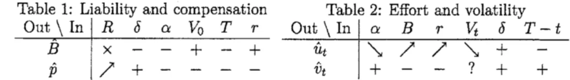
too complex to find them. Then we examine numerical

com-parative statics to find them. We compute $\hat{u}_{t}$,$\hat{v}_{t}$,

$\hat{B}$

, and $\hat{p}$ shifting $\alpha$,$r$,5,$B$, and $t$ for

fixed $V_{0}$,$T$, and$R$. Graphs and properties in detail

are

in Horikawa (2005) [3]. Numerical

results are as Table 1 and 2. The remarkable constructions are in conclusion.

Table 1: Liability and compensation Table 2: Effort and volatility

$\mathrm{O}\mathrm{u}\mathrm{t}\backslash \mathrm{I}\mathrm{n}\overline{B}\hat{p}$ $\nearrow R\mathrm{x}$ $+-\mathit{5}$ $–\alpha$ $V_{0}+-$ $-T-$ $-+r$ $\mapsto \mathrm{O}\iota 1\mathrm{t}u_{t}^{\mathrm{A}}[searrow]\nearrow\nearrow[searrow]+-\backslash \mathrm{I}\mathrm{n}\alpha BrV_{t}\delta T-t\hat{v}_{t}+--?++$

$\mathrm{O}\mathrm{u}\mathrm{t}\backslash \mathrm{I}\mathrm{n}$ $R$ 5 $\alpha$ $V_{0}$ $T$ $r$

$\overline{B}$

$\hat{p}$

$\mathrm{x}$ – – _$+$ – $+$

$\nearrow$ $+$ – – –

-$\bullet$ Arrows represent the analytical results. 7

means

not to yield

some

tendency.

Others express the numerical results.

4

Cash and Share Compensation

In this section, westudy

more

realisticcompensation

case:

it consists of fixed and variable

factors. The case only variable term is

we

have studied in the previous sections.

We let the priority for

a

shareholder at the maturity of liabilities

as

follows. A

share-holder first pay back her liabilities with interest rate $r$, that is, $Be^{rT}$

.

Next she_Pays her

manager some

fixed compensation $w$ from hershareholders’ equity. Here let$p\in[0, 1]$ the

ratio for her residual share. After she pays $w$ to him, she pays lOOp % of share as his

“incentive bonus.” Therefore we cannotjust compare $” p$” of this section to the

one

of the

previous sections. These

are

adjusted to the assumption ofMerton (1974) [5] at Section

2. We keep all the other setting andnotationsofour model

as we

have used. At last,

we

Then let

us

consider the problems of

a

manager and a shareholder respectively like

the section 3, The manager’sproblem is

$\max_{u,v}E[\ln\{w+p(V_{T}-(w+Be^{rT}))^{+}\}-\frac{1}{2}\int_{0}^{T}u_{t}^{2}dt]$

.

(8)

The shareholder’s problem is

$B,p,w\mathrm{m}\mathrm{a}\mathrm{x}$

$(1-p)E[(V_{T}-(w+Be^{rT}))^{+}]$ ,

$\mathrm{s}.\mathrm{t}$

.

_{$\max_{u,v}E[1\mathrm{r}$} $\{w+p(V_{T}-(w+Be^{rT}))^{+}\}-\frac{1}{2}\int_{0}^{T}u_{t}^{2}dt]\geq R$

,

(9)

$($\^u,

$\hat{v})\in \mathrm{a}\mathrm{r}\mathrm{g}\mathrm{m}\mathrm{x}(u,v)$

$E[\mathrm{I}\mathrm{n}$ $\{w+p(V_{T}-(w+Be^{rT}))^{+}\}-\frac{1}{2}\int_{0}^{T}u_{t}^{2}dt]$ , $p\in[0,1]$

.

Calculated Equation (8) and (9), we obtain the optimal solution

as

Theorem 3.

Theorem 3 (Optimal values when compensation includes fixed term).

Consider

the manager’s and shareholder$\prime s$ problem: Equation (8) and (9). We

assume

$\delta>0$

.

The optimal effort, volatility, the value

of

a

firm, and liabilities

are

$\hat{u}_{t}$ $=$ $\delta\check{z}_{t}e^{-\mu t}Z_{t}$,

$\hat{v}_{t}V_{t}$ $=$ $\alpha\tilde{H}_{t}\frac{\partial}{\partial y}g(t,\tilde{H}_{t})+\frac{\check{z}_{t}\delta^{2}Z_{t}}{\alpha}[\exp(s-t)-1]$ ,

$V_{t}$ $=$ $g(t, \tilde{H}_{t})-\frac{\check{z}_{t}\delta^{2}Z_{t}}{\alpha^{2}}[\exp\{\alpha^{2}(s-t)\}-1]$ ,

$\hat{B}$

$=$ $e^{-rT} \ovalbox{\tt\small REJECT}\frac{w}{p}+\frac{1}{N(d_{2}(t,\tilde{H}_{t}))}$

,

$[V_{t}- \tilde{H}_{t}N(d_{1}(t,\tilde{H}_{t}))-\frac{\check{z}_{t}\delta^{2}Z_{t}}{\alpha^{2}}[\exp\{\alpha^{2}(s-t)\}-1]]\ovalbox{\tt\small REJECT}$

.

where

$g(t,y)$ $:=$ $(\begin{array}{l}Be^{rT}-\underline{w}p\end{array})$$N(d_{2} (t, y))+yN(d_{1}(t,y))$,

$d_{1}(t,y)$ $:=$ $\frac{\ln(py/cw)+\alpha^{2}(T-t)/2}{\alpha\sqrt{T-t}}$,

$d_{2}(t,y)$ $:=$ $\frac{\ln(\mathfrak{M}/cw)-\alpha^{2}(T-t)/2}{\alpha\sqrt{T-t}}$,

$\tilde{H}_{t}$

$:=$ $\frac{1}{z_{t}Z_{t}\forall}$, $N(x):= \int_{-\infty}^{x}\frac{1}{\sqrt{2\pi}}\exp(-\frac{z^{2}}{2})dz$,

Remark

2.

We

cannot

compute the optimal compensation $\hat{p}$,

fixed

compensation

$\hat{w}$, and the range

of

reservation utility $R$ in Theorem3.

5

Conclusion

In thisPaper,

we

study the optimalliabilities of a firm, taking into account the incentive

of a manager. The risk neutral shareholders aim to maximize the value of a firm by

determining the level of liabilities and compensation to a manager. Forthese two factors,

a risk

averse

manager can improve the shareholders’ equity through his choice of effort

and volatility. Effort entails costwhereas volatility does not. Wederive theoptimaleffort,

volatility, liabilities, and compensation by

use

ofadynamic principal agent model

We mainlyfind the following three facts. Firstly, asmart managerdecreases liabilities

because he makes

a

large effort. Secondly,

an

efficient firm also decreases liabilities,

however it encourages a manager to make less effort. Finally, liabilities has an incentive

if effort ofa manager is valid, however it decreases as

a

firm grows.

Theseare somedirections that wecould extend in thispaper. Thefirst direction is the

analysis when compensation includes some fixed term $w$

.

Our difficulty dues to Remark

2. It would bring

more

fruitful result that whethertotry withinthe limitation of Remark

2

or

to try

more

relax condition. Other idea to be

more

realistic form is a non-linear

contract form. We

assume

that the compensation in

our

model is alinear contract. The

more

manager achieves, the

more

he obtain shares. That contracts yields a “call-option

form contract” in addition to a linear

one.

Now how do

we

solve it? We leave these

problemsfor ou$1\mathrm{r}$ further study.

References

[1] F. Black and M. Scholes. The pricing of options and corporate liabilities. Journal

_of

PoliticalEconomy, 81(3):637-654,

1973.

[2] A. Cadenillas, J. Cvitanic, and F. Zapatero. Leveragedecision and manager

compen-sation with choice of effort and volatility. Journal

_of

Financial Economics, 73:71-92,

2004.

[3] K. Horikawa. Optimal financial policy and incentive in afirm. Working Paper, Osaka

University, 2005.

[4] I. KaratzasandS. Shreve. Brownian Motion andStochasticCalculus. Springer-Verlag,

NY second edition, 1991.

[5] R. C. Merton. On thepricing of corporate debt: The risk structure of interest rates.

The Journal

_of

Finance, 29(2):449-470, May

1974.

[6] F. Modigliani and M. H. Miller. The cost of capital, corporation finance and the

theoryofinvestment. The

American

EconomicReview, 48(3):261-297, June

1958.

[7] E. Moreliec and C. W. Smith Jr. Investmentpolicy, financial policies, andthe control

ofagency conflicts. Working Paper, University

_of

Rochester, April 2004.

[8] B. Salanie. The Economics

_of

Contracts: A Primer. MIT Press, MA, second edition,