東北大学機関リポジトリTOUR

improvement evaluation of an electromagnetic

transducer utilizing a tuned inerter

著者

Keita Sugiura, Yuta Watanabe, Takehiko Asai,

Yoshikazu Araki, Kohju Ikago

journal or

publication title

Journal of vibration and control

volume

26

number

1-2

page range

56-72

year

2019-09-14

URL

http://hdl.handle.net/10097/00128297

performance improvement evaluation of

an electromagnetic transducer utilizing

a tuned inerter

Reprints and permission:

sagepub.co.uk/journalsPermissions.nav DOI: 10.1177/ToBeAssigned www.sagepub.com/

SAGE

Keita Sugiura

_{, Yuta Watanabe}

_{, Takehiko Asai}

_{, Yoshikazu Araki}

_{and Kohju Ikago}

Abstract

This research reports on the experimental verification of an enhanced energy conversion device utilizing a tuned inerter, called tuned inertial mass electromagnetic transducer (TIMET). The TIMET consists of a motor, a rotational mass, and a tuning spring. The motor and the rotational mass are connected to a ball screw and the tuning spring interfaced to the ball screw is connected to the vibrating structure. Thus, vibration energy of the structure is absorbed as electrical energy by the motor. Moreover, the amplified inertial mass can be realized by rotating relatively small physical masses. Therefore, by designing the tuning spring stiffness and the inertial mass appropriately, the motor can rotate more effectively due to the resonance effect, leading to more effective energy generation. The authors design a prototype of the TIMET and conduct tests to validate the effectiveness of the tuned inerter for electromagnetic transducers. Through excitation tests, the property of the hysteresis loops produced by the TIMET is investigated. Then a reliable analytical model is developed employing a curve fitting technique to simulate the behavior of the TIMET and to assess the power generation accurately. In addition, numerical simulation studies on a structure subjected to a seismic loading employing the developed model are conducted to show the advantages of the TIMET over a traditional electromagnetic transducer in both vibration suppression capability and energy harvesting efficiency.

Keywords

Energy harvesting, Structural control, Tuned inerter, Tuned inertial mass electromagnetic transducer, Mechatronics

Introduction

Vibratory energy harvesting technologies, which convert vibrational kinetic energy to electrical energy, have been getting attention over the last decade (Priya and Inman 2008;

Anton and Sodano 2007; Wei and Jing 2017). Traditionary, this research area has been focused on high-frequency vibration such as 10 Hz or higher on the order of millimeter amplitude. And the power harvested from such ambient vibration with piezoelectric devices has been limited to µW-mW scale for wireless sensing and embedded computing systems (Anton and Sodano 2007;Roundy et al. 2003; Beeby et al. 2006; Knight et al. 2008; Han et al. 2013). While, recently, energy harvesting employing electromagnetic devices from low-frequency oscillations has been getting attention (Drezet et al. 2018; Mahmoudi et al. 2014;Daqaq et al. 2009). Especially, for large-scale energy harvesting from a vibratory structure whose fundamental frequency is less than 10 Hz, an electromagnetic transducer (ET) employing a motor has been considered as an effective tool (Nagem et al. 1997; Zuo and Tang 2013). The ET is a device which converts mechanical energy of the linear motion to electrical energy by rotating a motor connected to a ball screw. The examples of these large-scale energy harvesting applications include railway systems (Nagode et al. 2010; Wang et al. 2012), automotive suspensions (Zuo et al. 2010;Abdelkareem et al. 2018), wave energy converters (Lattanzio and Scruggs 2011;

Liang and Zuo 2017), wind-excited high-rise buildings

(Tang et al. 2011), and wind-excited cable-stayed bridges (Shen and Zhu 2015;Jung et al. 2017;Jamshidi et al. 2017). These references have shown that ETs enable W-kW scale energy harvesting. In general, research activity to achieve further improvement of the ET aiming for W-kW scale energy harvesting has been devoted to developing power flow controllers for the motor (Cassidy and Scruggs 2013;

Cassidy et al. 2011b;Caruso et al. 2018).

Meanwhile, in the field of civil engineering, to improve the energy absorption performance in structures subjected to external loadings such as earthquakes and winds, tuned inertial mass has gotten a lot of attention recently (Ikago et al. 2012;Lazar et al. 2014). One of the examples is the tuned viscous mass damper consisting of two components, i.e., a rotational mass damper and a tuning spring parts (Ikago et al. 2012). The rotational mass damper is composed of a ball screw, a rotating mass, and a viscous material. The ball screw is employed to convert linear motion to rotational behavior and to produce an amplified equivalent inertial mass effect by rotating a relatively small physical

1_{University of Tsukuba, Japan} 2_{Nagoya University, Japan} 3_{Tohoku University, Japan}

Corresponding author:

Takehiko Asai, University of Tsukuba, 1-1-1 Tennodai, Tsukuba, Ibaraki 305-8573, Japan

mass. The force produced by the inertial mass is proportional to the relative acceleration between both ends, which is defined as inerter by Smith (2002). This rotational mass damper is connected to a vibrating structure through the tuning spring whose stiffness is tuned so that the inertial mass resonates with the natural frequency of the structure. Due to this tuned inerter effect, the energy absorption capability by the viscous material which is arranged in parallel with the rotational mass is increased.

By taking advantage of the tuned inerter, the tuned inertial mass electromagnetic transducer (TIMET) has been proposed by the authors to improve the energy harvesting performance of the ET (Asai et al. 2017). In this work, the authors proposed the parameter design method for the TIMET and examined the effective frequency bandwidth under broadband and narrowband random vibration inputs. Considering the fact that a ball screw is employed in both ETs and tuned viscous mass dampers, the TIMET can be realized through one ball screw, which makes the proposed device simple and compact. The authors investigated the potential of the TIMET not only as an energy harvester (Asai et al. 2017; Haraguchi and Asai 2017) but also as a structural control device for civil structures subjected to seismic loadings (Asai et al. 2018; Asai and Watanabe 2017) and the effectiveness was shown through numerical simulation studies. However, in these numerical simulation studies, energy loss occurring in the mechanical device was not considered, even though that could be a critical issue practically in the field of energy harvesting. While a device with the same mechanism as the TIMET, named tuned electromagnetic inertial mass damper, has been introduced byNakamura and Hanzawa(2017) independently from the authors, in which experimental studies were conducted. However, since the device was considered only as a structural control device, the power generation efficiency was not examined in the literature. Therefore, to investigate the possibility of the TIMET much further, experimental verification and development of a reliable analytical model considering the energy loss in the device are necessary for the assessment of the power generation performance.

This article makes a number of specific contributions, which extend results from recent conference paper by the authors (Watanabe et al. 2018). The primary objectives of this study are to design a prototype of the TIMET and to develop a reliable analytical model of the prototype including the mechanical energy loss in the device through experiments. In addition, the energy harvesting efficiency and structural control performance of the TIMET are evaluated using the developed model by comparing the conventional ET. In this paper, first, the mechanism of the proposed device of the TIMET is reviewed briefly along with the ordinary ET. Then a prototype device employing a three-phase permanent-magnetic synchronous motor (PMSM) designed by the authors is introduced. And experiments under various conditions are carried out using the prototype and the obtained results are shown. Subsequently, referring to the modeling method introduced in (Cassidy et al. 2011a) for the traditional ET, we seek the parameters for the analytical model of the prototype by the curve fitting technique to simulate the behavior of the TIMET accurately even when the motor is electronically controlled. Finally, to demonstrate

the structural control capability and the energy harvesting efficiency of the TIMET in comparison to the ET, numerical simulation studies using a single-degree-of-freedom (SDOF) system are conducted using the developed device models. Conclusions obtained from this study then follow.

Mechanism

In this section, the mechanism of the TIMET is introduced after the brief review of the ET. The equations of motion when the devices are attached to a base-excited SDOF oscillator are developed. Also, the damping induced by the motor as well as the generation power is formulated.

Electromagnetic transducer

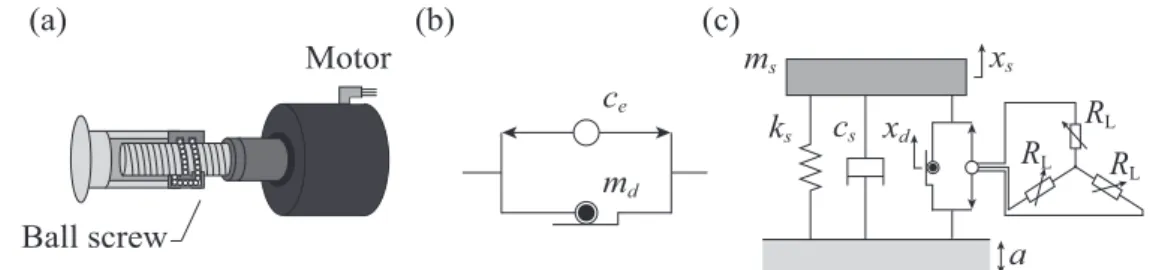
Figure 1(a) depicts the ET schematically. As illustrated, a three-phase motor is interfaced with a ball screw and mechanical energy of linear motion is converted to electrical energy by rotating the motor. This device can be modeled simply as shown in Fig. 1(b), in which md is the inertial

mass attributable to the motor and the ball screw and ceis

the damping coefficient caused by the motor. Let xdbe the

deformation of the ET, then the electromechanical force is defined as

fe=−cex˙d (1)

Thus the force produced by the ET is given by

ft= mdx¨d− fe (2)

Also the mechanical angle of the motor θmhas a relationship with xd; that is

θm= 2π

l xd (3)

where l is the lead conversion of the ball screw.

Next, consider the ET attached to a base-excited SDOF oscillator with three resistive loads as shown in Fig. 1(c). Let xs be the displacement of the mass of the oscillator

and assume that resistive loads RL are connected across the terminals of the motor. Then the equation of motion is developed as

msx¨s+ csx˙s+ ksxs=−msa− ft (4)

where ms, cs, and ksare the mass, damping, and stiffness

of the oscillator, respectively and a is the base acceleration. In this case, because the deformation of the ET corresponds to the displacement of the oscillator, we have xd= xs. Thus

from Eqs. (1) and (2), Eq. (4) would be

(ms+ md)¨xs+ (cs+ ce) ˙xs+ ksxs=−msa (5)

As stated above, this equation indicates that the motor rotates no more than the displacement of the mass of the oscillator in this system.

Tuned inertial mass electromagnetic transducer

The proposed TIMET is illustrated in Fig.2(a) schematically, which has the tuning spring and rotational mass producing additional inertial mass effect compared to the ET introduced above. The basic model of the TIMET can be represented as in Fig. 2(b). In a similar way to the ET case, let xd be the

Motor

Ball screw

c

m

k

c

R

R

R

a

x

(a)

(b)

(c)

m

x

Figure 1. ET: (a) Schematic illustration, (b) Model, (c) Attached to a base-excited oscillator with resistive loads.

Motor

Ball screw

Tuning spring

Rotational mass

m

c

k

m

k

c

R

R

R

a

x

(a)

(b)

(c)

x

Figure 2. TIMET: (a) Schematic illustration, (b) Model, (c) Attached to a base-excited oscillator with resistive loads.

deformation of the inertial mass part of the TIMET, then the force produced by the TIMET ftcan be expressed by Eq. (2)

as well. Because the tuning spring is connected in series, ft

is equal to the force by the tuning spring, so we also have

ft= kt(xs− xd) (6)

Form Eqs. (1), (2), and (6), we can derive the equation of motion of the inertial mass part given by

mdx¨d+ cex˙d+ ktxd− ktxs= 0 (7)

While the equation of motion for the oscillator with the TIMET has the form of Eq. (4) as well. And the deformation of the inertial mass part is not synchronized with the mass of the oscillator due to the tuning spring. Hence, let[xs xd

]T

be the displacement vector, then the equation of motion can be expressed as a 2DOF system in matrix form as

[ ms 0 0 md ] [ ¨ xs ¨ xd ] + [ cs 0 0 ce ] [ ˙ xs ˙ xd ] + [ ks+ kt −kt −kt kt ] [ xs xd ] =− [ ms 0 ] a (8) The advantage of the TIMET over the ordinary ET can be found when the excitation has the dominant frequency. Under this condition, the inertial mass can be resonated with the excitation at the specified frequency by designing the rotational mass and tuning spring stiffness appropriately. Then the deformation of the inertial mass could be larger than the displacement of the oscillator, leading to the increase in the rotation number of the motor and the energy harvesting performance is boosted. In this paper, it is shown experimentally that the TIMET can rotate the motor more efficiently to the excitation with the specified frequency through excitation tests.

Electromechanical modeling

To formulate the viscous damping coefficient ce and the

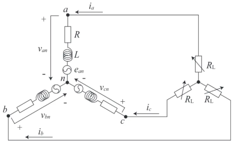
generated power Pgen by the motor, the circuit of the

star connected motor interfaced with three resistive loads represented in Fig. 3is considered here as inCassidy et al.

(2011a);McCullagh et al.(2016). Let ean, ebn, and ecnbe

the internal voltages for phase a, b, and c relative to the neutral node n. Then we have

eabc=   eeanbn ecn   =   cos(pθcos(pθm+m)23π) cos(pθm−2₃π )   Keθ˙m (9) where Keis the back-emf constant and p is the polarity of

the motor. Similarly, we define the line-to-neutral voltages at the terminals of the three phases and the corresponding line currents as vabc=   vvanbn vcn   , iabc=   iianbn icn   (10)

Then the dynamic equation for the three-phase motor becomes, in matrix form,

d dtiabc=

1

L(vabc− Riabc− eabc) (11)

where R and L are the line-to-neutral resistance and inductance of the motor, respectively. In this paper, we assume that the three phases have the same values for L and

R.

It is widely accepted to express the dynamics of the three-phase motor on the coordinate system consisting of quadrature (q), direct (d), and zero (0) (Pillay and Krishnan 1989). Thus vabcand iabccan be transformed to

vqd0= P (θm)vabc, iqd0= P (θm)iabc (12)

where P (θm) is the Park transformation defined as

P (θm) = √ 2 3   cos(pθm) cos(pθm+ 2 3π) cos(pθm− 2 3π) sin(pθm) sin(pθm+2₃π) sin(pθm−2₃π)

1 √ 2 1 √ 2 1 √ 2   (13)

-R

R

R

R

L

i

i

v

v

v

e

i

a

b

c

n

Figure 3. Electrical schematic for the three-phase motor with resistive loads.

By this transformation, the number of phases is reduced from three to two because

v0= 0, i0= 0 (14) are satisfied due to Kirchhoff’s law, applied at the neutral node, i.e.,

ia+ ib+ ic= 0 (15)

Also, it should be noted that this transformation does not change the norm, i.e.,

|vabc| = |vqd0|, |iabc| = |iqd0| (16)

Substituting Eq. (12) into Eq. (11) gives

d

dtiqd0− Q ˙θmiqd0=

1

L(vqd0− Riqd0− P (θm)eabc)

(17) where the matrix Q is

Q = ( d dθm P (θm) ) P−1(θm) = p   01 −1 00 0 0 0 0   (18) and the dynamics of the motor is described by three differential equations d dtiq= 1 L ( −Riq+ vq− p ˙θmLid− √ 3 2Ke ˙ θm ) d dtid= 1 L(−Rid+ vd+ p ˙θmLiq) d dti0= 1 L(−Ri0+ v0) (19)

Finally, because the torque provided by the motor is √

3

2Keiq and the lead conversion is 2π

l , the

electromechani-cal force feis given as

fe= √ 3 2 2π l Keiq (20)

Now, we consider the circuit illustrated in Fig.3, in which three resistive loads in a star connection are attached to the motor. With this configuration we have

vabc=−RLiabc i.e., vqd0=−RLiqd0 (21)

Substitute the second equation of Eq. (21) into Eq. (17), then

iqand idcan be expressed as

d dtiq = 1 L ( −(R + RL)iq− p ˙θmLid− √ 3 2Ke ˙ θm ) d dtid= 1 L ( −(R + RL)id+ p ˙θmLiq ) (22)

Furthermore, under the assumption that ˙θmis slowly varying,

iqand idare approximated asCassidy et al.(2011a)

iq =− √ 3 2 (R + RL)Keθ˙m (R + RL)2+ (p ˙θmL)2 , id=− √ 3 2 (p ˙θmL)Keθ˙m (R + RL)2+ (p ˙θmL)2 (23)

From these expressions, the dynamics of id can be

neglected under the condition that p ˙θm≪ (R + RL)/L. This condition is satisfied for the experiments presented in the next section, thus in this article, iq and id can be

approximated further as iq =− √ 3 2 Keθ˙m R + RL , id= 0 (24)

Therefore, the electromechanical force fe is obtained by

substituting the first equation of Eq. (24) into Eq. (20) as

fe=− 3πK2 e l(R + RL) ˙ θm=− 6π2_K2 e l2_{(R + R} L) ˙ xd (25)

Hence the damping coefficient provided by the motor would be ce= 6π2_K2 e l2_{(R + R} L) (26) Additionally, for this article, the generated power by the motor is equal to the dissipated power by the resistive loads

RL, which is defined as

Pgen= (i2a+ i2b+ i2c)RL (27) Thus, from Eqs. (16) and (24), the generated power is also expressed as

Pgen= i2qRL=

3RL(Keθ˙m)2 2(R + RL)2

Table 1. Design parameters Parameter Value Ke 0.584 Nm/Arms p 5 R 0.69 Ω L 1.92 mH l 20 mm kt 39240 N/m

Experimental characterization

To identify the characteristics of the TIMET introduced above experimentally, a prototype of the proposed device is designed and excitation testings are conducted. The hysteresis loops produced by the ET and TIMET are compared and analytical models of the prototype devices are developed based on the sine sweep wave test in this section.

Device design and experimental setup

The designed prototype and the experimental setups in which the prototype is connected to the electric servo actuator are shown in Fig. 4(a) and (b). The motor employed for power generation in this research is a SGMJ-08A three-phase PMSM by YASKAWA and a precision ball screw manufactured by THK is used. The parameters for the motor, tuning spring, and ball screw of the prototype are summarized in Table 1. The rotational mass and tuning spring of the prototype are designed to be removable, which enables the device to be used as an ET as well. As shown in Fig.4(c), the rotational mass part consists of a rotational plate and six round shape weights, therefore the produced inertial mass can be adjustable by changing the radius of rotation of the six weights. The rotational plate has three different radii which can produce three different inertial mass values, i.e., Type T-1, T-2, and T-3. For Type T-1, the weights are fixed to the inner six holes on the rotational plate, the middle six holes for T-2, and the exterior six holes for T-3. As for the tuning spring, four compression springs are used for the prototype. These springs are at free length when the device is at the static equilibrium position and only two of the springs are compressed depending on the direction and apply restoring force when the inertial mass or the actuator are displaced from the static equilibrium position.

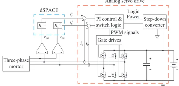
In this study, the resistive load configuration is realized by connecting the three-phase motor to an analog servo drive as inCassidy and Scruggs(2013). This concept is illustrated by the block diagram in Fig.5. The three-phase servo drive that is used in this study is an SX30A8 analog servo drive from Advanced Motion Controls. One of the advantages of this drive is that four-quadrant regenerative operation is available, i.e., the servo drive is capable of not only dissipating but also injecting power. The servo drive requires command signals for two of the three phases which are denoted by

i∗_a and i∗_b in Fig. 5. And the command for the third phase is determined by enforcing the relationship given by Eq. (15) in the servo drive. Tracking of the desired command signals is achieved through high-frequency PWM switching control of six MOSFETs. The switching frequency of the

servo drive used here is 27 kHz. The output voltages of the three-phase motor are measured by a dSPACE MicroLabBox data acquisition system at a sample rate of 1 kHz and two of the phases of the line-to-neutral voltages denoted by vanand

vbn are divided by the desired load resistance RL and the obtaining current command signals i∗_a and i∗_b are sent to the servo drive.

Sine wave excitation tests

To demonstrate the force capabilities of the ET and TIMET, external forces are applied to the devices by the electric servo actuator as shown in Fig.4(a) and (b). Applied forces are measured by the load cell installed between the actuator and the device and the displacements and accelerations are measured by laser displacement sensors and accelerometers, respectively. For the TIMET case, the displacement and acceleration of the inertial mass are measured separately from the input displacement and acceleration as shown in Fig.4(b). To obtain the velocity data for the input and the inertial mass part, the encoders embedded in the motors for the electrical servo actuator and for power generation are used, respectively.

Figure6presents the forces measured by the load cell for the ET cases to 1.0 Hz sine wave input with an amplitude of 15 mm. The previously introduced analog servo drive is employed to simulate various resistive loads including 10, 3, and 1 Ω in addition to the open circuit case, i.e., RL=∞. As can be seen in Fig.6(b), the ET exhibits almost viscous damping behavior and shows larger damping force as the load resistance becomes smaller.

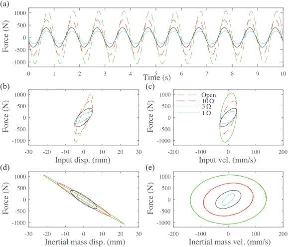
On the other hand, the forces produced by the TIMET with Type T-1 inertial mass are shown in Fig.7. The input sine wave is 1.0 Hz as well, while 5 mm input amplitude is used instead to ensure that the amplified inertial mass displacement due to resonance effect would not exceed the deflection limit of the tuning springs. The load resistance values are set to 10, 3, 1 Ω, and open as well. Comparing Fig.

7(b) and (d), we can find that the displacement of the inertial mass part is amplified compered to the input displacement. At the same time, the amplification of the velocity can be confirmed by comparing Fig. 7(c) and (e), which leads to the improvement of the energy absorbing capability of the TIMET. We can observe that the inertial mass produces negative stiffness in Fig. 7(d). It should be noted that the open case produces larger force than any other case. This is because the open case induces larger displacement of the inertial mass because of the lower damping.

Sine sweep wave test

To further examine the resonance effect of the inertial mass part of the TIMET and the effective frequency bandwidth, we input a sine sweep wave ranging from 0.6 to 1.1 Hz over 100 s. To clearly observe the difference of the resonance behaviors of the TIMET among the three different inertial masses, i.e., Type T-1, T-2, and T-3, the displacement amplitude of the input sine sweep wave is set to 3 mm and the velocity amplitude varies gradually with the change of the input frequency. The time histories of the displacement and frequency of the input sine sweep wave to the TIMET

(a)

(b)

(c)

Tuning spring

Rotational mass

Actuator

Laser disp.

sensor 1

_{sensor 2}

Laser disp.

Motor

Load cell

Ball screw

Laser disp.

sensor

Accelerometor 1

Accelerometor 2

Accelerometor

Figure 4. Photographs of the designed prototype and experimental setup: (a) ET, (b) TIMET, (c) Rotational mass.

R

_R

PI control &

switch logic

PWM signals

Gate drives

Three-phase

mortor

Logic

Power

_Step-down

converter

v

v

i

i

i

i

Analog servo drive

dSPACE

Figure 5. Three-phase motor interface with a dSPACE and an analog servo drive.

0 1 2 3 4 5 6 7 8 9 10

Time (s)

F

orc

e (N

)

Input disp. (mm)

F

orc

e (N

)

Input vel. (mm/s)

F

orc

e (N

)

(a)

(b)

(c)

Figure 6. Forces of the electromagnetic transducer for various load resistances to 1 Hz sine wave with an amplitude of 15 mm: (a)

0 1 2 3 4 5 6 7 8 9 10

Time (s)

F

orc

e (N

)

Input disp. (mm)

F

orc

e (N

)

Input vel. (mm/s)

F

orc

e (N

)

Inertial mass disp. (mm)

F

or

ce

(

N

)

Inertial mass vel. (mm/s)

F

or

ce

(

N

)

(a)

(b)

(c)

(d)

(e)

Figure 7. Forces of the TIMET for various load resistances to 1 Hz sine wave with an amplitude of 5 mm: (a) Force vs. time, (b)

Force vs. input displacement, (c) Force vs. input velocity, (d) Force vs. inertial mass displacement, (e) Force vs. inertial mass displacement.

are presented in Fig.8. The terminals of the motor are left open for this test.

The responses of the inertial mass displacement for Type T-1, T-2, and T-3 are compared with the input amplitude of 3 mm in Fig.9. As can be observed in the figure, Type T-1, T-2, and T-3 reach their peak amplitudes around 67 s, 46 s, and 30 s, respectively, indicating that their resonance frequencies are 0.93 Hz, 0.83 Hz, and 0.75 Hz, respectively. Also, at these frequencies, the amplitudes of these three open circuit cases approach almost 30 mm, which are 10 times as large as the input of 3 mm due to resonance. Considering the fact that the ET does not amplify the input amplitude, we can conclude that the tuned inerter amplifies the displacement and improves the power generation in a specified frequency range. However, it should be noted that the response of the Type 3 goes below the input amplitude around 80 s corresponding to about 1 Hz. Therefore, these sine sweep wave tests confirm that appropriate parameter design considering the target frequency is necessary to make the best use of the TIMET. In addition, it is shown that the effective frequency bandwidth can be adjusted by changing the radius of the weight for the rotational mass.

Parameter fit and model verification

Finally, analytical models and their parameter values for the designed prototype are developed from the experimental data by the curve fitting technique based on the least squares method. To take the wide range of input frequency to the

device into account, the previously presented results obtained from the sine sweep wave tests are employed. The terminals of the motor are left open, i.e., ce= 0. Also, to develop more

accurate analytical models than the models shown in Figs.

1(b) and2(b), the detailed models depicted in Fig.10 are considered. In these models, viscous dampings ct and cd

that are present in the location of the tuning spring and the ball screw mechanism are added. In addition, a Coulomb friction term fc is included to represent the friction force

acting on the device. The data used for curve fitting are downsampled to 100 Hz and the least square fitting method within MATLAB is implemented to solve for the optimal parameters in the model.

In particular, for the TIMET cases, to determine the parameter values for the model shown in Fig.10(b), the force equilibrium relationship given by

f = ct( ˙xs− ˙xd) + kt(xs− xd)

= mdx¨d+ (ce+ cd) ˙xd+ fcsgn( ˙xd)

(29)

should be considered. Solving Eq. (29) for ¨xdresults in

¨ xd= 1 md{c t( ˙xs− ˙xd) + kt(xs− xd) − (ce+ cd) ˙xd− fcsgn( ˙xd)} (30)

where xd and ˙xd can be calculated through numerical

-40 -20 0 20 40

D

is

p. (m

m

)

Time (s)

F

re

q. (H

z)

(a)

(b)

Figure 8. Time history of the sine sweep applied to the devices: (a) Displacement, (b) Frequency.

0 10 20 30 40 50 60 70 80 90 100

Time (s)

D

is

p. (m

m

)

Figure 9. Responses of the inertial mass displacement of the TIMET for the open circuit.

(a)

(b)

k

c

m

c

c

f

m

c

c

f

Figure 10. Detailed models: (a) ET, (b) TIMET.

to the differential equation. Then the force given by Eq. (29) is evaluated by the least squares method.

The obtained parameter values for the TIMET are summarized in Table 2 as well as the ET case, in which 40171 N/m, 39690 N/m, and 40479 N/m are obtained for the tuning spring stiffness kt for each TIMET case. We

can confirm that these values for all three cases are very close to the nominal value of 39240 N/m given in Table1, which verifies the accuracy of the parameters predicted by the curve fitting technique. In addition, the results reflects the difference of the inertial mass md for the TIMETs as

intended. Moreover, the resonance frequencies calculated by fr= 1 2π √ kt md (31) become 0.91 Hz, 0.80 Hz, and 0.72 Hz, respectively and these values are matched well with the resonant frequencies observed in the sine sweep wave tests. However, the obtained values for ct, cd, and fcare relatively high, indicating that the

undesirable energy loss occurred in the mechanical device is non-negligible.

The curve produced by the obtained analytical model for Type T-1 is compared with the experimental data in Fig.11. As can be seen, not only the force but also the inertial mass displacement by the developed model show good agreement with the experimental data with the input frequency range of 0.6 to 1.1 Hz.

In addition to the graphical comparison between the experimental data and the developed model, a quantitative study of the errors proposed by Spencer et al. (1997) is conducted. First, let fi and ˆfi be the ith element of the

experimentally measured force vector and the ith element of the force vector by the developed model using Eq. (29), respectively. Then error norms for time, displacement, and velocity can be calculated by

Et= (∑n i=1(fi− ˆfi) 2)1/2 (∑n_i=1(fi− µf)2) 1/2, Exs = (∑n i=1(fi− ˆfi)2| ˙xs,i| )1/2 (∑n_i=1(fi− µf)2) 1/2 , Ex˙s = (∑n i=1(fi− ˆfi)2|¨xs,i| )1/2 (∑n_i=1(fi− µf)2) 1/2 (32)

where n is the number of data, µf is the mean value of

the measured force, ˙xs,i is the ith element of the input

measured velocity, ¨xs,i is the ith element of the measured

input acceleration. Moreover, for the TIMET cases, the error norms with respect to the inertial mass displacement and velocity can be defined as

Exd= (∑n i=1(fi− ˆfi) 2_{| ˙x} d,i| )1/2 (∑n_i=1(fi− µf)2) 1/2 , Ex˙d= (∑n i=1(fi− ˆfi) 2_|¨x d,i| )1/2 (∑n_i=1(fi− µf)2) 1/2 (33)

where ˙xd,i is the ith element of the measured velocity of

the inertial mass, ¨xd,i is the ith element of the measured

acceleration of the inertial mass. The error norms calculated by Eqs. (32) and (33) are listed in Table3. The error norms calculated for the TIMET models are smaller than those calculated for the ET model considered.

Response to a fluctuating electromechanical

force

The data examined previously are based on the responses of the device when the load resistance to the motor is held at

a constant value. However, to maximize the performance of the proposed device, the load resistance should be controlled depending on the response. Thus, it should be shown that the developed model can simulate the behavior of the device accurately when the electronics introduces an additional fluctuating electromechanical force, which is given by Eq. (1). In this article, two tests are carried out to validate the accuracy of the proposed model with a fluctuating electromechanical force, i.e., (1) constant RL, random displacement; and (2) random RL, random displacement.

In the first test conducted to verify the model, the device is excited with the random displacement as shown in Fig.12(a). And a constant load resistance RL= 10 Ω is simulated by using the analog servo drive. The response of the TIMET with Type T-1 inertial mass to this test is compared with the predicted response in Fig.13. As can be seen, the model predicts the behavior of the device with satisfactory accuracy. For this test, the error norms given by Eq. (32) are calculated to be Et= 0.0411, Exs = 0.0041, Ex˙s = 0.0097, Exd=

0.0071, and Ex˙d= 0.0148

For the second verification test, the load resistance is simulated randomly by the analog servo drive as shown in Fig. 12(b). The upper bound on the resistance load is 200 Ω and the lower bound is 1 Ω. And the same random displacement as in Fig. 12(a) is applied to the device. The response produced by the developed model for the TIMET with Type T-1 inertial mass is compared with the experimental data in Fig. 14. Slight discrepancies can be found in the figure, however, the model predicts the experimental data with satisfactory accuracy. For this test, the error norms calculated by Eqs. (32) and (33) deteriorate to Et= 0.1313, Exs = 0.0131, Ex˙s= 0.0302,

Exd= 0.0232, and Ex˙d= 0.0591.

Response analyses

As stated before, one of the promising applications of the TIMET can be found in the field of structural control such as a vibration suppression control device for the structures subjected to earthquake loadings. To evaluate the effectiveness of the TIMET compared to the ET, a base-exited SDOF structure as shown in Figs. 1(c) and 2(c) subjected to an earthquake record is considered in this section. Numerical simulation studies using the developed models in the previous section are carried out and the 1995 JMA Kobe record shown in Fig.15is employed as an input acceleration a.

The mass, stiffness, and damping for the SDOF structure model used in this study are ms= 12400 kg, cs= 2505

Ns/m, and ks= 316266 N/m, respectively. These values are

determined based on the design method introduced for the tuned viscous mass damper in Ikago et al. (2012) so that the structure model suits to the developed model for the TIMET with Type T-1 inertial mass. In particular, the viscous damping factor for the structure and the mass ratio defined by

ζs= cs 2√msks , µ =md ms (34) are set to ζs= 0.02 and µ = 0.1, respectively. Assuming that

the damping provided by the TIMET is the summation of

Table 2. Parameters obtained from the curve fitting method. Parameter ET TIMET T-1 T-2 T-3 md 23.5 kg 1240 kg 1567 kg 1998 kg kt N/A 40171 N/m 39690 N/m 40479 N/m ct N/A 112 Ns/m 203 Ns/m 147 Ns/m cd 313 Ns/m 356 Ns/m 285 Ns/m 427 Ns/m fc 22.6 N 18.2 N 22.7 N 20.8 N 0 10 20 30 40 50 60 70 80 90 100

Time (s)

F

orc

e (N

)

Input disp. (mm)

F

orc

e (N

)

Input vel. (mm/s)

F

orc

e (N

)

Inertial mass disp. (mm)

F

orc

e (N

)

Inertal mass vel. (mm/s)

F

orc

e (N

)

Time (s)

Ine

rt

ia

l m

as

s di

sp. (m

m

)

(a)

(b)

(c)

(d)

(e)

(f)

Figure 11. Comparisons of the force and inertial mass displacement of the TIMET (T-1) for the sine sweep test: (a) Force vs. time,

(b) Force vs. input displacement, (c) Force vs. input velocity. (d) Force vs. inertial mass displacement, (e) Force vs. inertial mass velocity, (f) Inertial mass displacement vs. time.

(2012) can be written as kt= (βωs)2md, ce+ cd = 2βζωsmd (35) where ωs= √ ks ms , β = 1− √ 1− 4µ 2µ , ζ = √ 3(1−√1− 4µ) 4 (36)

Then the parameters of the SDOF structure is determined so that the above equations are satisfied. Taking cd= 356

Ns/m in Table 2 into account, RL= 3.72 Ω, i.e., ce=

2544 Ns/m calculated by Eq. (26) is chosen for this study. Thus this can be considered as an example of constant RL and random displacement input. Also, the natural frequency of the structure determined by ωs becomes 5.05 rad/s,

-5 0 5

D

is

p. (m

m

)

Time (s)

R

(Ω

)

(a)

(b)

Figure 12. Random inputs: (a) Displacement, (b) Resistance load.

0 2 4 6 8 10 12 14 16 18

Time (s)

F

orc

e (N

)

Input disp. (mm)

F

orc

e (N

)

Input vel. (mm/s)

F

orc

e (N

)

Inertial mass disp. (mm)

F

or

ce

(

N

)

Inertial mass vel. (mm/s)

F

or

ce

(

N

)

Time (s)

Ine

rt

ia

l m

as

s di

sp. (

m

m

)

(a)

(b)

(c)

(d)

(e)

(f)

Figure 13. Comparisons between the experiment and model of the TIMET (T-1) for the constantRLand random displacement

test: (a) Force vs. time, (b) Force vs. input displacement, (c) Force vs. input velocity. (d) Force vs. inertial mass displacement, (e) Force vs. inertial mass velocity, (f) Inertial mass displacement vs. time.

0 2 4 6 8 10 12 14 16 18

Time (s)

F

orc

e (N

)

Input disp. (mm)

F

orc

e (N

)

Input vel. (mm/s)

F

orc

e (N

)

Inertial mass disp. (mm)

F

or

ce

(

N

)

Inertial mass vel. (mm/s)

F

or

ce

(

N

)

Time (s)

Ine

rt

ia

l m

as

s di

sp. (

m

m

)

(a)

(b)

(c)

(d)

(e)

(f)

Figure 14. Comparisons between the experiment and model of the TIMET (T-1) for the randomRLand random displacement test:

(a) Force vs. time, (b) Force vs. input displacement, (c) Force vs. input velocity. (d) Force vs. measured inertial mass displacement, (e) Force vs. measured inertial mass velocity, (f) Inertial mass displacement vs. time.

0 5 10 15 20 25

Time (s)

A

cc

el

. (m

/s

)

Figure 15. Ground acceleration of the 1995 JMA Kobe.

i.e., 0.80 Hz, which is within the frequency range used for developing model. Therefore, the reliability of result produced by the developed device model for this simulation study is guaranteed.

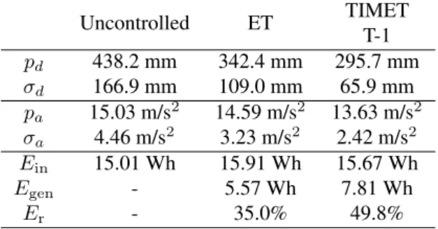
The response results obtained from the developed models are summarized in Table 4. For comparison, no control device case is carried out in addition to the ET and TIMET

cases. In this table, pd and σd are the peak and root mean

square (RMS) of the displacements of the structure and pa

and σaare the peak and RMS of the absolute accelerations.

Table 3. Error norms for the the sine sweep test

Error norm ET TIMET

T-1 T-2 T-3 Et 0.3151 0.0261 0.0470 0.0482 Exs 0.0553 0.0027 0.0047 0.0045 Ex˙s 0.1967 0.0064 0.0107 0.0105 Ex˙d N/A 0.0063 0.0095 0.0088 Ex˙d N/A 0.0183 0.0246 0.0219

Table 4. Results to the 1995 JMA Kobe record.

Uncontrolled ET TIMET T-1 pd 438.2 mm 342.4 mm 295.7 mm σd 166.9 mm 109.0 mm 65.9 mm pa 15.03 m/s2 14.59 m/s2 13.63 m/s2 σa 4.46 m/s2 3.23 m/s2 2.42 m/s2 Ein 15.01 Wh 15.91 Wh 15.67 Wh Egen - 5.57 Wh 7.81 Wh Er - 35.0% 49.8%

energy Egen, and the energy conversion ratio Erdefined as

Ein=− ∫ tf 0 msa ˙xsdt, Egen= ∫ tf 0 Pgendt, Er= Egen Ein (37) respectively, are provided in the table as well. Note that

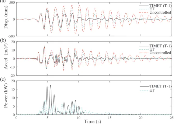
tf is 25 s. The time history responses of the displacement,

acceleration, and the generated power given by Eq. (28) are plotted in Fig.16. The result summarized in Table4 shows that the conversion ratios are 35.0% for the ET and 49.8% for the TIMET, indicating that the TIMET can convert larger portion of the input energy to electricity than the ET despite the existence of the energy loss in the device. Additionally, we can confirm that the TIMET suppresses the peak response values more and decays the responses more quickly than the ET from Fig.16.

Conclusions

In this research, the prototype of the proposed TIMET was designed and its behavior and energy conversion performance were examined through excitation tests. The results obtained from the sine sweep wave tests showed that the TIMET can increase the number of rotations of the motor around the specified frequency in comparison with the ET and that the specified frequency was adjusted by changing the inertial mass value. Also, the reliable analytical models including the mechanical energy loss in the prototype were developed based on the sine sweep wave tests with the wide frequency range using the curve fitting technique. The models with the obtained parameters provided good agreement with the experimental responses of the device under a various operating conditions, including constant load resistance with random displacement and random load resistance with random displacement, which showed the accuracy of the developed model.

Furthermore, this article compared the structural control capabilities and energy harvesting efficiencies of the developed device models installed in the SDOF structure subjected to the 1995 JMA Kobe record through numerical simulation studies. And the result showed the superiority of the TIMET over the ET in both vibration suppression, i.e., response displacement and acceleration, and power generation senses. However, the obtained models indicated that the undesirable energy dissipation in the device were still relatively high compared with the energy absorbed by the motor. Thus, for future work, to enhance the energy conversion efficiency of the device much further, we seek to develop a device for reducing energy loss. At the same time, to make the most of the TIMET, appropriate algorithms to control the power flow for the motor which is applicable even to nonlinear systems and mechanisms to adjust the inertial mass value automatically in response to changes in the frequency of the external input should be incorporated into the system.

Acknowledgements

This research was supported financially by JSPS KAKENHI Grant number 17H04942 which is gratefully appreciated. Also, the authors would like to thank Dr. Nakaminami and Dr. Kida of Aseismic Devices Co. Ltd. and Mr. Chikamoto of THK CO., LTD. for their help in designing the prototype device used in this research.

References

Abdelkareem MA, Xu L, Ali MKA, Elagouz A, Mi J, Guo S, Liu Y and Zuo L (2018) Vibration energy harvesting in automotive suspension system: A detailed review. Applied Energy 229: 672 – 699. DOI:https://doi.org/10.1016/j.apenergy.2018.08.030. Anton SR and Sodano HA (2007) A review of power harvesting

using piezoelectric materials (2003-2006). Smart Materials and Structures 16(3): R1.

Asai T, Araki Y and Ikago K (2017) Energy harvesting potential of tuned inertial mass electromagnetic transducers. Mechanical

Systems and Signal Processing 84, Part A: 659 – 672. DOI:

10.1016/j.ymssp.2016.07.048.

Asai T, Araki Y and Ikago K (2018) Structural control with tuned inertial mass electromagnetic transducers. Structural Control

and Health Monitoring 25(2): e2059. DOI:10.1002/stc.2059.

Asai T and Watanabe Y (2017) Outrigger tuned inertial mass electromagnetic transducers for high-rise buildings subject to long period earthquakes. Engineering Structures 153: 404 – 410. DOI:10.1016/j.engstruct.2017.10.040.

Beeby SP, Tudor MJ and White NM (2006) Energy harvesting vibration sources for microsystems applications. Measurement

Science and Technology 17(12): R175.

Caruso G, Galeani S and Menini L (2018) Semi-active damping and energy harvesting using an electromagnetic transducer.

Journal of Vibration and Control 24(12): 2542–2561. DOI:

10.1177/1077546316688993.

Cassidy I, Scruggs J, Behrens S and Gavin HP (2011a) Design and experimental characterization of an electromagnetic transducer for large-scale vibratory energy harvesting applications.

Journal of Intelligent Material Systems and Structures 22(17):

-500 0 500

D

is

p. (m

m

)

A

cc

el

. (m

/s

)

Time (s)

P

ow

er (kW

)

(a)

(c)

(b)

Figure 16. Comparisons of the time histories: (a) Response displacement, (b) Response acceleration, (c) Power generation.

Cassidy IL and Scruggs JT (2013) Nonlinear stochastic controllers for power-flow-constrained vibratory energy harvesters.

Jour-nal of Sound and Vibration 332(13): 3134 – 3147.

Cassidy IL, Scruggs JT and Behrens S (2011b) Optimization of partial-state feedback for vibratory energy harvesters subjected to broadband stochastic disturbances. Smart Materials and

Structures 20(8): 085019. DOI:10.1088/0964-1726/20/8/

085019.

Chopra A (2007) Dynamics of Structures. Prentice-Hall international series in civil engineering and engineering mechanics. Pearson Education. ISBN 9788131713297. Daqaq MF, Stabler C, Qaroush Y and Seuaciuc-Osorio T (2009)

Investigation of power harvesting via parametric excitations.

Journal of Intelligent Material Systems and Structures 20(5):

545–557. DOI:10.1177/1045389X08100978.

Drezet C, Kacem N and Bouhaddi N (2018) Design of a nonlinear energy harvester based on high static low dynamic stiffness for low frequency random vibrations. Sensors and Actuators A:

Physical 283: 54 – 64. DOI:https://doi.org/10.1016/j.sna.2018.

09.046.

Han B, Vassilaras S, Papadias CB, Soman R, Kyriakides MA, Onoufriou T, Nielsen RH and Prasad R (2013) Harvesting energy from vibrations of the underlying structure. Journal

of Vibration and Control 19(15): 2255–2269. DOI:10.1177/

1077546313501537.

Haraguchi R and Asai T (2017) Numerical verification of the tuned inertial mass effect of a wave energy converter. In:

Smart Materials, Adaptive Structures and Intelligent Systems,

volume 1. American Society of Mechanical Engineers, p. V001T07A003. DOI:10.1115/SMASIS2017-3772.

Ikago K, Saito K and Inoue N (2012) Seismic control of single-degree-of-freedom structure using tuned viscous mass damper.

Earthquake Engineering & Structural Dynamics 41(3): 453–

474. DOI:10.1002/eqe.1138.

Jamshidi M, Chang C and Bakhshi A (2017) Self-powered hybrid electromagnetic damper for cable vibration mitigation. Smart

Structures Systems 20(3): 285–301. DOI:10.12989/sss.2017.

20.3.285.

Jung HY, Kim IH and Jung HJ (2017) Feasibility study of the electromagnetic damper for cable structures using real-time hybrid simulation. Sensors 17(11).

Knight C, Davidson J and Behrens S (2008) Energy options for wireless sensor nodes. Sensors 8(12): 8037. DOI:10.3390/ s8128037.

Lattanzio SM and Scruggs JT (2011) Maximum power generation of a wave energy converter in a stochastic environment. In: Control Applications (CCA), 2011 IEEE International

Conference on. pp. 1125–1130. DOI:10.1109/CCA.2011.

6044428.

Lazar IF, Neild S and Wagg D (2014) Using an inerter-based device for structural vibration suppression. Earthquake Engineering

& Structural Dynamics 43(8): 1129–1147. DOI:10.1002/eqe.

2390.

Liang C and Zuo L (2017) On the dynamics and design of a two-body wave energy converter. Renewable Energy 101: 265 – 274. DOI:https://doi.org/10.1016/j.renene.2016.08.059. Mahmoudi S, Kacem N and Bouhaddi N (2014) Enhancement

of the performance of a hybrid nonlinear vibration energy harvester based on piezoelectric and electromagnetic transduc-tions. Smart Materials and Structures 23(7): 075024. DOI: 10.1088/0964-1726/23/7/075024.

McCullagh JJ, Scruggs JT and Asai T (2016) Vibration energy harvesting with polyphase AC transducers. In: Proc. SPIE, volume 9799. pp. 9799 – 9799 – 13. DOI:10.1117/12.2225458. Nagem R, Madanshetty S and Medhi G (1997) An electromechani-cal vibration absorber. Journal of Sound and Vibration 200(4): 551 – 556. DOI:https://doi.org/10.1006/jsvi.1996.0681.

Nagode C, Ahmadian M and Taheri S (2010) Effective energy harvesting devices for railroad applications. In: Proc. SPIE, volume 7643. pp. 76430X–76430X–10. DOI:10.1117/12. 847866.

Nakamura Y and Hanzawa T (2017) Performance-based placement design of tuned electromagnetic inertial mass dampers.

Frontiers in Built Environment3: 26. DOI:10.3389/fbuil.2017.

00026.

Pillay P and Krishnan R (1989) Modeling, simulation, and analysis of permanent-magnet motor drives. i. the permanent-magnet synchronous motor drive. IEEE Transactions on Industry Applications 25(2): 265–273. DOI:10.1109/28.25541.

Priya S and Inman D (2008) Energy Harvesting Technologies. Springer US. ISBN 9780387764641.

Roundy S, Wright PK and Rabaey J (2003) A study of low level vibrations as a power source for wireless sensor nodes.

Computer Communications 26(11): 1131 – 1144. DOI:10.

1016/S0140-3664(02)00248-7.

Shen W and Zhu S (2015) Harvesting energy via electromagnetic damper: Application to bridge stay cables. Journal of Intelligent Material Systems and Structures 26(1): 3–19. DOI:

10.1177/1045389X13519003.

Smith MC (2002) Synthesis of mechanical networks: the inerter.

IEEE Transactions on Automatic Control 47(10): 1648–1662.

DOI:10.1109/TAC.2002.803532.

Spencer BF, Dyke SJ, Sain MK and Carlson JD (1997) Phenomenological model for magnetorheological dampers.

Journal of Engineering Mechanics 123(3): 230–238. DOI:

10.1061/(ASCE)0733-9399(1997)123:3(230).

Tang X, Zuo L and Kareem A (2011) Assessment of energy potential and vibration mitigation of regenerative tuned mass dampers on wind excited tall buildings. In: the ASME 2011

International Design Engineering Technical Conferences and Computers and Information in Engineering Conference, 18.

Washington, DC, pp. 333–342.

Wang JJ, Penamalli GP and Zuo L (2012) Electromagnetic energy harvesting from train induced railway track vibrations. In: Proceedings of 2012 IEEE/ASME 8th IEEE/ASME

International Conference on Mechatronic and Embedded Systems and Applications. pp. 29–34. DOI:10.1109/MESA.

2012.6275532.

Watanabe Y, Sugiura K and Asai T (2018) Experimental verification of a tuned inertial mass electromagnetic transducer. In: Proc.

SPIE, volume 10595. pp. 10595 – 10595 – 13. DOI:10.1117/

12.2295867.

Wei C and Jing X (2017) A comprehensive review on vibration energy harvesting: Modelling and realization. Renewable and

Sustainable Energy Reviews 74: 1 – 18. DOI:https://doi.org/10.

1016/j.rser.2017.01.073.

Zuo L, Scully B, Shestani J and Zhou Y (2010) Design and characterization of an electromagnetic energy harvester for vehicle suspensions. Smart Material Structures 19(4): 045003. DOI:10.1088/0964-1726/19/4/045003.

Zuo L and Tang X (2013) Large-scale vibration energy harvesting.

Journal of Intelligent Material Systems and Structures 24(11):