BAT AGN Spectroscopic Survey. XI. The Covering
Factor of Dust and Gas in Swift/BAT Active
Galactic Nuclei
著者
Kohei Ichikawa, Claudio Ricci, Yoshihiro Ueda,
Franz E Bauer, Taiki Kawamuro, Michael J Koss,
Kyuseok Oh, David J Rosario, Shimizu T. Taro,
Marko Stalevski, Lindsay Fuller, Christopher
Packham, Benny Trakhtenbrot
journal or
publication title
The Astrophysical Journal
volume
870
number
31
page range
1-16
year
2019-01-02
URL
http://hdl.handle.net/10097/00126934
doi: 10.3847/1538-4357/aaef8fBAT AGN Spectroscopic Survey. XI. The Covering Factor of Dust and Gas in
Swift/BAT
Active Galactic Nuclei
Kohei Ichikawa1,2,3,4 , Claudio Ricci5,6,7 , Yoshihiro Ueda8 , Franz E. Bauer9,10 , Taiki Kawamuro11,19 , Michael J. Koss12 , Kyuseok Oh8,19 , David J. Rosario13 , T. Taro Shimizu14 , Marko Stalevski15,16 , Lindsay Fuller2,
Christopher Packham2,11, and Benny Trakhtenbrot17,18
1
Department of Astronomy, Columbia University, 550 West 120th Street, New York, NY 10027, USA;[email protected]
2
Department of Physics and Astronomy, University of Texas at San Antonio, One UTSA Circle, San Antonio, TX 78249, USA 3
Frontier Research Institute for Interdisciplinary Sciences, Tohoku University, Sendai, Miyagi 980-8578, Japan 4
Astronomical Institute, Tohoku University, Aramaki, Aoba-ku, Sendai, Miyagi 980-8578, Japan 5
Núcleo de Astronomía de la Facultad de Ingeniería, Universidad Diego Portales, Av. Ejército Libertador 441, Santiago, Chile 6
Kavli Institute for Astronomy and Astrophysics, Peking University, Beijing 100871, People’s Republic of China 7
Chinese Academy of Sciences South America Center for Astronomy, Camino El Observatorio 1515, Las Condes, Santiago, Chile 8
Department of Astronomy, Kyoto University, Oiwake-cho, Sakyo-ku, Kyoto 606-8502, Japan 9
Millennium Institute of Astrophysics(MAS), Nuncio Monseñor Sótero Sanz 100, Providencia, Santiago, Chile 10
Space Science Institute, 4750 Walnut Street, Suite 205, Boulder, CO 80301, USA 11
National Astronomical Observatory of Japan, 2-21-1 Osawa, Mitaka, Tokyo 181-8588, Japan 12Eureka Scientific, 2452 Delmer Street Suite 100, Oakland, CA 94602-3017, USA 13
Centre for Extragalactic Astronomy, Department of Physics, Durham University, South Road, DH1 3LE Durham, UK 14
Max-Planck-Institut für extraterrestrische Physik, Postfach 1312, D-85741, Garching, Germany 15
Astronomical Observatory, Volgina 7, 11060 Belgrade, Serbia 16
Sterrenkundig Observatorium, Universiteit Gent, Krijgslaan 281-S9, Gent B-9000, Belgium 17
Department of Physics, ETH Zurich, Wolfgang-Pauli-Strasse 27, CH-8093 Zurich, Switzerland 18
School of Physics and Astronomy, Tel Aviv University, Tel Aviv 69978, Israel
Received 2018 March 7; revised 2018 October 12; accepted 2018 November 2; published 2019 January 2 Abstract
We quantify the luminosity contribution of active galactic nuclei (AGNs) to the 12 μm, mid-infrared (MIR; 5–38 μm), and total IR (5–1000 μm) emission in the local AGNs detected in the all-sky 70 month Swift/Burst Alert Telescope(BAT) ultrahard X-ray survey. We decompose the IR spectral energy distributions (SEDs) of 587 objects into the AGN and starburst components using templates for an AGN torus and a star-forming galaxy. This enables us to recover the emission from the AGN torus including the low-luminosity end, down to
- -
(L )
log 14 150 erg s 1 41, which typically has significant host galaxy contamination. The sample demonstrates that the luminosity contribution of the AGN to the 12μm, the MIR, and the total IR bands is an increasing function of the 14–150 keV luminosity. We also find that for the most extreme cases, the IR pure-AGN emission from the torus can extend up to 90μm. The total IR AGN luminosity obtained through the IR SED decomposition enables us to estimate the fraction of the sky obscured by dust, i.e., the dust covering factor. We demonstrate that the median dust covering factor is always smaller than the median X-ray obscuration fraction above an AGN bolometric luminosity of log(Lbol(AGN) erg s-1)42.5. Considering that the X-ray obscuration fraction is equivalent to the covering factor coming from both the dust and gas, this indicates that an additional neutral gas component, along with the dusty torus, is responsible for the absorption of X-ray emission.
Key words: galaxies: active– galaxies: nuclei – infrared: galaxies Supporting material:figure set, machine-readable table
1. Introduction
One of the fundamental open questions of extragalactic astrophysics is how supermassive black holes (SMBHs) and their host galaxies coevolve(e.g., Alexander & Hickox2012). Active galactic nuclei (AGNs) are the best targets for understanding this process of coevolution, because they are in the stage where mass accretion onto SMBHs occurs with the release of large amounts of radiation (e.g., Yu & Tremaine 2002; Marconi et al. 2004), until they reach their maximum achievable mass ofMBH 1010.5M(Netzer2003;
McLure & Dunlop2004; Trakhtenbrot2014; Jun et al.2015; Inayoshi & Haiman2016; Ichikawa & Inayoshi2017).
Ultrahard (E>10 keV) X-ray observations are one of the most reliable methods for identifying AGNs. Thanks to the
combination of (1) a strong penetration power up to
-
(N )
log H cm 2 24 (e.g., Ricci et al.2015) and (2) the high contrast with stellar X-ray emission (e.g., Mineo et al.2012), ultrahard X-ray surveys allow an unbiased census of AGNs up to Compton-thick levels (e.g., Koss et al. 2016). Among the recent available surveys, Swift/BAT provides the most sensitive X-ray survey of the whole sky in the 14–195 keV range, reaching aflux level of (1.0–1.3)×10−11erg s−1cm−2 in thefirst 70 months of operations (Baumgartner et al.2013), and a deeper flux of (7.2–8.4)×10−12erg s−1cm−2 in the recently updated 105 month catalog(Oh et al.2018).
Infrared(IR) observations also provide an effective method to study AGNs because the central engine of an AGN is expected to be surrounded by a dusty “torus” (Krolik & Begelman 1986), which is heated by the AGN and re-emits thermally in the mid-IR (MIR) (e.g., Gandhi et al. 2009;
© 2019. The American Astronomical Society. All rights reserved.
19
Ichikawa et al. 2012, 2017; Asmus et al. 2015). A recent upward revision of black hole scaling relations (Kormendy & Ho 2013) indicates that the local mass density in black holes should be higher, suggesting that a larger population of heavily obscured AGN gas and dust is required tofill the mass gap of the revised local black hole mass density (e.g., Novak 2013; Comastri et al. 2015). These populations contribute signifi-cantly to the infrared background (e.g., Murphy et al. 2011; Delvecchio et al. 2014), especially in the MIR band (Risaliti et al. 2002). However, since star formation from the host galaxy sometimes contaminates the MIR emission, especially for low-luminosity AGNs with L14 150- <1043erg s−1 (e.g.,
Ichikawa et al. 2017), and the torus is too compact (<10 pc; e.g., Jaffe et al.2004) to be fully resolved (e.g., García-Burillo et al. 2016; Imanishi et al. 2018), the precise estimation of AGN thermal activity is not straightforward.
Fortunately,several methods have been proposed to isolate the emission from the torus from the starburst component. One of them is to use MIR observations with high spatial resolution (∼0 3–0 7) to resolve the starburst emission of the host galaxies down to scales of 10 pc (Packham et al. 2005; Radomski et al.2008; Hönig et al.2010; Alonso-Herrero et al. 2011,2016; Ramos Almeida et al.2011; González-Martín et al. 2013; Asmus et al. 2014; Ichikawa et al. 2015; Martínez-Paredes et al. 2017). In addition, the advent of IR interfero-metric observations, with their exquisite resolving power(with baselines up to 130 m), has spatially resolved the dusty nuclear regions and shown that their outer radii in the MIR are typically several parsecs (e.g., Jaffe et al. 2004; Raban et al. 2009; Burtscher et al.2013). Notably, some show the polar elongated dust emission suggestive of a dusty outflow (Hönig et al.2012, 2013; Tristram et al.2014; López-Gonzaga et al.2016, Leftley et al.2018). However, because of the limited sensitivity and the spatial resolution of current telescopes (see a recent review by Burtscher et al.2016), these two methods are available only for a few tens of bright sources located in the very local universe (z<0.01). Another possible approach is to separate the spectral emission of the AGN and the starburst (SB) component. Multiple decomposition methods have been applied to MIR spectra, mainly using aromatic features as a proxy for star formation(e.g., Tran et al.2001; Lutz et al.2004; Sajina et al.2007; Alonso-Herrero et al.2012; Ichikawa et al. 2014; Hernán-Caballero et al. 2015; Kirkpatrick et al. 2015; Symeonidis et al. 2016), to broadband IR spectral energy distributions(SEDs, e.g., da Cunha et al.2008; Hatziminaoglou et al.2008; Xu et al.2015; Lyu et al.2016,2017; Shimizu et al. 2017),and to the combination of both spectra and SEDs (e.g., Mullaney et al.2011). The advantage of the SED decomposi-tion is that it is less affected by the differing spatial resoludecomposi-tions inherent in aperture photometry, and can be applied to high-z sources(e.g., Stanley et al.2015; Lyu et al.2016; Mateos et al. 2016) and/or to large (N>100) samples, for which MIR imaging and spectroscopy with high spatial resolution would require significant amounts of time on large-diameter (>8 m) telescopes.
In this paper, we decompose the IR SEDs of the ultrahard X-ray-selected Swift/BAT 70 month AGN catalog (Baumgart-ner et al.2013) into AGN and host galaxy components. Thanks to intensive follow-up observations by BAT AGN Spectro-scopic Survey20(BASS; Koss et al.2017; Lamperti et al.2017;
Ricci et al.2017b), we are able to obtain reliable information on the gas column density (NH), absorption-corrected
14–150 keV X-ray luminosity, and black hole mass (MBH) of
the sample.
The main goal of this work is to quantitatively assess the AGN contribution to the 12μm band, MIR (5–38 μm) band, and total IR (5–1000 μm) band down to log(L14 150- erg s-1)41 in order to investigate torus (1) the correlation between MIR and X-ray luminosity and (2) the dust covering factor of the torus, minimizing issues related to host galaxy contamination. Through-out the paper, we adopt standard cosmological parameters (H0=70.0 km s−1Mpc−1,ΩM=0.3, and ΩΛ=0.7).
2. Sample
Our initial sample is based on the sample of Ichikawa et al. (2017), which contains the 606 non-blazar AGNs from the Swift/BAT 70 month catalog (Baumgartner et al. 2013) at galactic latitudes ( >∣ ∣b 10) for which secure spectroscopic redshifts are available. In this study, we use the column density (NH) and the absorption-corrected 14–150 keV luminosity
(L14–150) tabulated in Ricci et al. (2017b). They are also
summarized in Table1.
In Ichikawa et al. (2017), we reported the 3–500 μm IR counterparts for our AGN sample, utilizing the IR catalogs obtained from WISE (Wright et al.2010; Cutri et al.2013), AKARI(Murakami et al.2007), IRAS (Beichman et al.1988), and Herschel(Griffin et al.2010; Poglitsch et al. 2010). Out of the 606 sources, we identified 604, 560, 601, and 402 counterparts in the total IR, near-IR(NIR; <5 μm), MIR, and far-IR (FIR; 60–500 μm) bands, respectively. The reader should refer to Ichikawa et al. (2017) for details of the IR catalogs. While Ichikawa et al. (2017) compiled the representativefluxes at 12, 22, 70, and 90 μm, by combining similar wavelength bands in the multiple IR catalogs listed above, in this study we regard each IR band with a different central wavelength as independent photometry. Therefore, there are at most 17 available IR photometric bands between 3 and 500μm, as identified in Table1. For the data points with the same wavelengths(i.e., 12, 25, 60, 100, and 160 μm), the adopted photometry was chosen based on the priorities reported in the IR catalog of Ichikawa et al.(2017) to measure the IR emission from both nucleus and host galaxy in a uniform way for the entire AGN sample. The 12μm flux density was obtained with the following priority: WISE, IRAS/Point Source Catalog (PSC), and IRAS/Faint Source Catalog(FSC). For the 25, 60, and 100 μm flux densities, on the other hand, we followed a different order(IRAS/PSC and IRAS/FSC), while for the 160 μm flux density we used Herschel/PACS and, when not available, AKARI/FIS. The corrected data are obtained from a wide range of different angular resolutions from Herschel/PACS (70 μm; 6 arcsec) to IRAS/FIR (100 μm; ≈1 arcmin). Using nearly the same sample, Mushotzky et al.(2014) already showed that the bulk of PACS 70μm is point-like at the spatial resolution of Herschel, suggesting that the FIR emission from the host galaxy is really compact (with a median value of 2 kpc FWHM) and unresolvable for most of our sample. Thus, we conclude that the aperture dependence with more moderate resolutions obtained by AKARI and IRAS is negligible(see also Meléndez et al. 2014; García-González et al. 2016a; Ichikawa et al.2017; Lutz et al.2018).
20
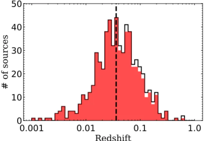
To acquire IR SEDs with a number of data points sufficient for spectral decomposition we require, for each source, at least three photometric bands within the rest-frame 3–500 μm. This is because three data points are needed to define the normal-ization of the two components (AGN torus and host galaxy). Applying this criterion, our sample is reduced to 588 sources. In addition, we require at least one data point from either the NIR or FIR band to estimate the host galaxy component, which brings the sample to 587 sources. This is thefinal sample used for this study, and it represents a large fraction of the initial sample (587/606=97%). The redshift distribution of the sample is shown in Figure1.21
We divide the sample into two AGN types based on NH
obtained by Ricci et al. (2017b). We define the AGNs with <
NH 1022cm−2 as unobscured AGNs, and those with
NH 1022cm−2 as obscured ones. Overall we have 300 unobscured and 287 obscured AGNs. The AGN types for the complete BAT 70 month catalog are tabulated in Ricci et al. (2017b), as well as in Table1. We note that Koss et al.(2017) found a 95% agreement for the unobscured and obscured AGNs with the presence of a broad Hβ line for optical types Seyfert 1–1.8 and Seyfert 2.
3. Analysis
We decompose the IR SEDs of AGNs using SB and AGN templates to estimate the intrinsic AGN IR luminosity. We use the IDL script DecompIR coded by Mullaney et al.(2011) and
Table 1
Column Descriptions for the IR Catalog of the Swift/BAT 70 Month AGN Survey
Col.# Header Name Format Unit Description
1 objID string L Swift/BAT ID as shown in Baumgartner et al. (2013)
2 ctpt1 string L optical counterpart name
3 z float L redshift
4 NH_log float L logarithmic column density(log(NH/cm-2))
5 lbat_log float L absorption-corrected logarithmic 14–150 keV luminosity (log(L14-150/erg s-1)) 6 lbol_const_log float L logarithmic bolometric AGN luminosity(log(Lbol(AGN) erg s-1))
7 lbol_log float L logarithmic bolometric AGN luminosity(log(Lbol(M04) erg s-1)) using Marconi et al. (2004) 8(9) fnu3p4_(err)_fqualmod float Jy 3.4μmprofile-fitting flux density (error) obtained from WISE
10(11) fnu4p6_(err)_fqualmod float Jy 4.6μmprofile-fitting flux density (error) obtained from WISE 12(13) fnu9a_(err)_fqualmod float Jy 9.0μmflux density (error) obtained from AKARI/IRC 14(15) fnu12wipf_(err)_fqualmod float Jy 12μmflux density (error)
16 fnu12wipcatalog string L reference catalogs for 12μm: W=WISE, Ip=IRAS/PSC, If=IRAS/FSC 17(18) fnu18a_(err)_fqualmod float Jy 18.0μmflux density (error) obtained from AKARI
19(20) fnu22w_(err)_fqualmod float Jy 22μmprofile-fitting flux density (error) obtained from WISE 21(22) fnu25ipf_(err)_fqualmod float Jy 25μmflux density (error)
23 fnu25ipfcatalog string L reference catalogs for 25μm: Ip=IRAS/PSC, If=IRAS/FSC 24(25) fnu60ipf_(err)_fqualmod float Jy 60μmflux density (error)
26 fnu60ipfcatalog string L reference catalogs for 60μm: Ip=IRAS/PSC, If=IRAS/FSC 27(28) fnu65a_(err)_fqualmod float Jy 65μmflux density (error) obtained from AKARI/FIS 29(30) fnu70p_(err)_fqualmod float Jy 70μmflux density (error) obtained from Herschel/PACS 31(32) fnu90a_(err)_fqualmod float Jy 90μmflux density (error) obtained from AKARI/FIS 33(34) fnu100ipf_(err)_fqualmod float Jy 100μmflux density (error)
35 fnu100ipfcatalog string L reference catalogs for 100μm: Ip=IRAS/PSC, If=IRAS/FSC 36(37) fnu140a_(err)_fqualmod float Jy 140μmflux density (error) obtained from AKARI/FIS 38(39) fnu160pa_(err)_fqualmod float Jy 160μmflux density (error)
40 fnu160pacatalog string L reference catalogs for 160μm: P=Herschel/PACS, A=AKARI/FIS 41(42) fnu250s_(err)_fqualmod float Jy 250μmflux density (error) obtained from Herschel/SPIRE
43(44) fnu350s_(err)_fqualmod float Jy 350μmflux density (error) obtained from Herschel/SPIRE 45(46) fnu500s_(err)_fqualmod float Jy 500μmflux density (error) obtained from Herschel/SPIRE 47 l12_AGN_afSta15_log float L logarithmic decomposed 12μm AGN luminositylog(L(m ) erg s-)
12 mAGN 1 48 lMIR_AGN_afSta15_log float L logarithmic decomposed MIR AGN luminositylog(L( ) erg s-)
MIRAGN 1
49 lIR_AGN_afSta15_log float L logarithmic decomposed total IR luminositylog(L( ) erg s-)
IRAGN 1
50 l12AGNratio_afSta15 float L f( m )
AGN 12 m 51 AGNpercentage_MIR_afSta15 float L fAGN(MIR) 52 AGNpercentage_afSta15 float L fAGN(IR)
53 flag_upperlimit int L flag of AGN: detection (= 0), upper limit (= 1), and lower-limit (= −1) 54 R_Sta16_afSta15_log float L logR=log(L( ) L( ))
IRAGN bolAGN 55 CF_Sta16_tau9p7eq3_afSta15 float L C dustT( )
56 SBtemplate_afSta15 string L SB template used for the SEDfitting this study: SB1–SB5 Note.The detail of the selection of theflux is compiled in Section2. The full catalog is available as a machine readable electronic table. (This table is available in its entirety in machine-readable form.)
21M81 is not shown in thefigure due to its very low redshift of z=10−4 (Ricci et al.2017b).
further developed by Del Moro et al.(2013). This code accepts IR photometry points in the 3–500 μm range as input and properly accounts for the filter and instrument response functions of the photometry points. It then computes the approximate levels of AGN and host galaxy contributions by fitting data that combine a host galaxy component with an AGN. DecompIR contains the mean AGN template produced from the Swift/BAT 9 month catalog (Tueller et al. 2008), which broadly traces the typical spectral forms of face-on and edge-on clumpy torus models (e.g., Nenkova et al. 2008a, 2008b) as shown in Mullaney et al. (2011). It also includes the five star-forming galaxy templates (Mullaney et al.2011; Del Moro et al.2013), using the average starburst SEDs derived by Dale et al.(2001). The five galaxy templates are composites of local star-forming galaxies with LIR <1012L (Brandl et al. 2006). They characterize well the full range of host galaxy SED shapes(Del Moro et al.2013; Stanley et al.2015), such as the galaxy template library of Chary & Elbaz(2001). Using these representative templates, we are able to fit the data without suffering from the degeneracy of the fitting procedure caused by the large number of templates. In addition, some of our sources have only three data points, so it is reasonable to keep the number of free parameters as small as possible.
The free parameters of the fitting are the normalizations of the AGN and host galaxy templates; therefore at least three IR data points are needed tofit the SEDs. However, we added one more free parameter for only the very luminous sources. It is known that, in high-luminosity AGNs, the IR SEDs become muchflatter at shorter wavelengths, which could be related to the stronger radiation field heating the surrounding dust to higher temperatures than in moderate-luminosity AGNs (e.g., Richards et al.2006; Netzer et al.2007; Mullaney et al.2011; Symeonidis et al.2016; Lani et al.2017; Lyu et al.2017). Our AGN SEDs also show such a tendency, especially at high luminosities (L14 150- >1044erg s−1). Therefore, for the sources that have at least four data points and luminosities
>
-L14 150 1044erg s−1, we also allow the spectral indexα1of
the AGN template(see Mullaney et al.2011) to be shallower at wavelengths shorter than 19μm.
To determine the bestfitting parameters, we first fit the SED by using the five host galaxy templates (SB1–SB5) and the AGN template. We then check the results obtained using the five different SB templates, and we choose the one that
provides the best results according to the chi-squared statistic (χ2) minimization.
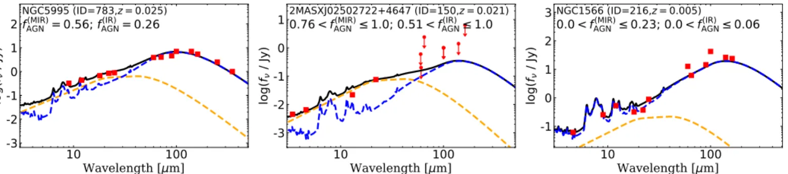
Figure 2 shows examples of the best-fitting SEDs that include both the AGN and star formation components, together with the best-fitting SEDs that require only the host galaxy or the AGN component. All the other SEDs of our sample are compiled in the online journal. Overall, 474 sources required both the AGN and the host galaxy templates, while 94 sources required only the AGN template. For the latter objects, the fitting quality does not improve even when including an additional SB template. Since most of those sources(89 out of 94) are not detected in the FIR bands, and considering that the FIR bands have shallower sensitivities than the MIR ones, the lack of a significant contribution of the SB template in the MIR does not always imply that the host galaxy does not contribute to the total IR luminosity. In order to assess how much the host galaxy could contribute to the total infrared luminosity without affecting the observed SEDs, we calculate the upper limits on the contribution from star formation by following Stanley et al. (2015), where the same SED decomposition routine, DecompIR, was used. This was done by increasing the normalization of the host galaxy template until it reached one of the upper limits or exceeded the 3σ uncertainty of a data point. We then used the star-forming galaxy template that gave the highest value of IR luminosity as our conservative upper limit. For the sources that have an upper limit on the host galaxy component, we show the lower limits of the AGN contribution to the MIRflux (5–38 μm;
( )
fAGNMIR) and to the total IR flux (5–1000 μm; fAGN(IR)) in each SED,
as illustrated in the middle panel of Figure2. The lower limits on
( )
fAGNMIR and fAGN(IR) are reported in Table1, and readers can use the flag (flag_limit) to assess whether the values are lower limits or not.
There are 18 sources in our sample that were bestfit to the host galaxy template alone (fAGN(MIR)=0). Again, in order to
assess the contribution of AGNs to the total IR luminosity, we calculate the upper limits on the contribution from the AGN torus with the same methods as for the AGN-dominated SEDs, as discussed above. The upper limits of fAGN(MIR) and fAGN(IR) are also shown in the right panel of Figure2(see also Table1).
Using this SEDfitting approach, we have measurements of the AGN luminosity in the 12μm (L12 m(AGNm )), MIR (LMIR(AGN)), and
total IR(LIR(AGN)) bands. All the values, as well as the IR flux
densities, are tabulated in Table1. We do not compile the IR star-forming luminosity, due to the impossibility of obtaining reliable estimates for the sources not detected in the FIR.
4. Results and Discussion
4.1. Fractional Luminosity Contribution of AGNs to the IR Band
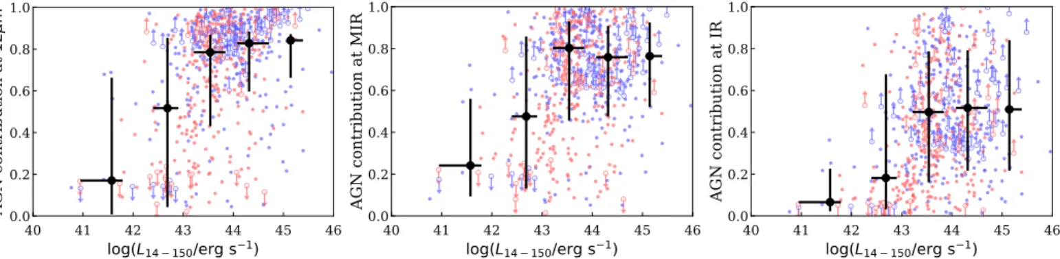
Figure3shows the median of the AGN contributions to the 12μm, MIR, and total IR luminosities as a function of L14–150.
The AGN contribution is calculated from the ratio of the AGN luminosity to the total(SF plus AGN) luminosity:
= + m m m m ( ) ( ) ( ) ( ) ( ) ( ) f L L L . 1 AGN 12 m,MIR,IR 12 m,MIR,IR AGN 12 m,MIR,IR AGN 12 m,MIR,IR SF
Figure3shows that the luminosity contribution of the AGNs to the 12μm, MIR, and total IR bands increases with L14–195. At the low-luminosity end (L14 195- <1043erg s−1), Figure 3 indicates that the host galaxy emission significantly Figure 1.Redshift distribution of AGNs in the Swift/BAT 70 month catalog at
Galactic latitude of∣ ∣b >10(black solid line: 606 objects; see also Ichikawa et al.2017) and of those used in this study (red area: 587 objects). The vertical
contaminates(;50%–80%) the 12 μm and MIR bands. At the high-luminosity end(L14 195- >1043erg s−1), it clearly shows
that the AGN component is the dominant (80%) energy source at 12μm and in the MIR band. This overall result is broadly consistent with previous studies that explored the AGN contribution using imaging with high spatial resolution (e.g., Asmus et al.2011,2014, and references therein). These works are discussed in AppendixA.1. On the other hand, in the total IR band, the AGN component contributes only up to ;50% even at high luminosities. This result is consistent with the calculations done for local quasars(Lyu et al.2017), where it is shown that AGNs contribute ;50% of the flux even if they provide 90% of the MIR emission.
Figure 3 also shows that the scatter of the percentage is ∼20% for f( )
AGN
MIR and increases up to ∼35% for f( ) AGN
IR . The
scatter is mostly due to AGN-dominated sources without any detections in the FIR bands. Since no distant sources with z>0.05 have been observed with Herschel (see Meléndez et al. 2014; Shimizu et al. 2016), those sources have very shallow upper limits: 0.2 Jy at 60μm (IRAS/FSC) and/or 0.55 Jy at 90μm (AKARI/FIS). This allows a possible contribution of the host galaxy emission to the FIR bands, even when its contribution to the MIR flux is negligible as discussed in Section3(see also Lyu & Rieke2017). Therefore, FIR photometry with higher sensitivity is crucial to quantify the host galaxy contribution for those sources.
4.2. IR Pure-AGN Candidates
Some sources show AGN-dominated SEDs even in the FIR bands. These sources are called IR pure-AGN(Mullaney et al. 2011; Rosario et al. 2012, 2018; Matsuoka & Woo 2015; Ichikawa et al.2017), and they are ideal candidates for deriving intrinsic AGN IR templates. These IR pure-AGN have a spectral turnover at 20–40 μm (Alonso-Herrero et al. 2012; Hönig et al. 2014; Fuller et al. 2016; Lopez-Rodriguez et al. 2018) and a declining flux density from 40 μm to 160 μm, suggesting a very low contribution from the starburst in the host galaxy. In order to check the SED turnover quantitatively, we plot IR color–color plots of f70μm/f160μmversus f22μm/f70μm
in Figure4. Bothflux ratios are known to be sensitive to the SED peak, and therefore to the dust temperature (Meléndez et al.2014; García-González et al.2016b). The orange shaded area in Figure 4 ( f70μm/f160μm>1.0 and f22μm/f70μm>1.0)
indicates a decline influx density as a function of wavelength from 22μm to 160 μm since the sources fulfill f22μm> f70μm>f160μm.
Figure4 also shows the simulated IR color as a function of
( )
fAGNIR for the each SB template. All IR colors follow a similar trend: f22μm/f70μmincreases up to f22μm/f70μm;1.0 with fAGN(IR)
up to 0.9, while f70μm/f160μm shows a very shallow increase until fAGN(IR)0.8. However, for fAGN(IR)>0.9, f70μm/f160μmstarts
to drastically increase, reaching values up to ;7.0. Thus, sources located in the orange shaded area should have AGN-dominated IR SEDs with fAGN(IR) >0.90. In this study we define a source as IR pure-AGN when it fulfills the following criteria: (1) f( ) >
0.90
AGN
IR and (2) a significant detection at both
60–70 μm and 160 μm. A total of nine sources are selected with these criteria, and they are shown with the black crosses in Figure 4. Most IR pure-AGN are successfully located in the orange shaded area in the color–color plot. Figure5shows the SEDs of the nine selected IR pure-AGN. All sources show an SED turnover between;20 μm and ;70 μm, a declining flux density from 70μm to 160 μm, and no FIR bump due to star formation up to 90μm, with the exception of Fairall9 and II SZ 010. Some of the sources in our sample have already been reported as being dominated by emission from the torus in the IR from the study of their Spitzer/IRS spectra (e.g., MCG–05-23-16; Ichikawa et al.2015), based on the spectral turnover at 20–40 μm (Alonso-Herrero et al. 2012; Hönig et al. 2014; Fuller et al.2016; Lopez-Rodriguez et al.2018).
We also check the AGN properties of IR pure-AGN compared to the parent sample. The means and standard deviations of the logarithmic X-ray luminosity, black hole mass, and Eddington ratio of this subsample are álogL14 150- ñ =43.70.3
álogMBHñ = 7.80.5, andáloglEddñ = -1.20.3,
respec-tively. These values are consistent with those of the parent sample of álogL14 150- ñ = 43.70.8, álogMBHñ =8.00.8,
and áloglEddñ = -1.50.8. This result suggests that the dominant contribution of AGNs to the total IR band is not related to their higher AGN luminosities, lower BH masses, or higher Eddington ratio, while it implies that they have weaker star formation luminosities than other AGNs of similar luminosity. Actually, MCG–05-23-16 is one of the pure IR-AGN whose CO emission has not been detected(Rosario et al. 2018) in the Swift/BAT AGN subset of the LLAMA survey (Davies et al.2015). This suggests that its host galaxy already
Figure 2.Example of our IR SEDs and their best-fit models. The orange and blue dashed curves represent fitted the AGN and host galaxy templates, respectively. The black solid curve is the combination of AGN and host galaxy templates, while the red squares with error bars are theflux densities. Each panel also shows the object ID based on the Swift/BAT 70 month catalog, the redshift, and the luminosity contribution of the AGNs to the MIR (f( )
AGNMIR) and IR bands (fAGN(IR)). Left panel: an example of a source showing both AGN and host galaxy contributions. Middle panel: an example of an AGN torus-dominated SED. The host galaxy template is plotted as an upper limit. Right panel: an example of a source with a host galaxy-dominated SED, with the AGN template plotted as an upper limit. The complete figure set of all SEDs of our sample (587 images) is available in the online journal.
lacks the molecular gas to produce the star formation. The ongoing molecular gas observations conducted by the BASS survey (M. Koss et al. 2018, in preparation) will explore the origin of the deficit of star formation in these IR pure-AGN sources.
4.3. Correlation between the 12 mm AGN and 14–150 keV Luminosities
Figure 6 shows the relation between L12 m(AGNm ), LMIR(AGN), and L14–150 in the range 1040erg s−1<L14–150<1047erg s−1. Blue and red crosses represent unobscured and obscured AGNs, respectively. The upper limits, shown as open circles, represent the host galaxy-dominated sources that have a possible AGN contribution in the 12μm and MIR bands as discussed in Section3. The slope of the relation betweenL(m )
12 m
AGN,L( ) MIR
AGN, and
L14–150is estimated considering the two variables as independent
parameters. Since our data contain both detections and upper limits, we apply the survival analysis method using the Python package22 ASURV (Feigelson & Nelson 1985; Isobe et al. 1986; Lavalley et al.1992) to account for the upper limits on
m ( )
L12 mAGN and LMIR(AGN). We use the slope bisector fits, which
minimize the perpendicular distance from the slope line to data points. Thefits, with the form oflog(L12 m,MIR(m ) /10 erg s-)
AGN 43 1 =
D + D
(a a) (b b) log(L14 150- /1043erg s-1), where Δa
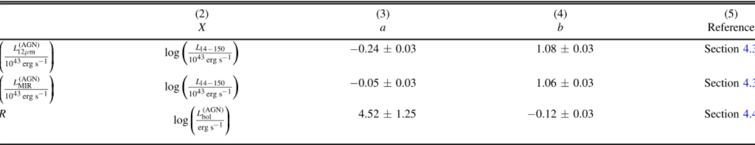
and Δb are the standard deviations of a and b, respectively, result in = - + ´ m -( ) ( ) ( ) ( ) L L log 10 erg s 0.24 0.03 1.08 0.03 log 10 erg s , 2 12 m AGN 43 1 14 150 43 1 = - + ´ -( ) ( ) ( ) ( ) L L log 10 erg s 0.05 0.03 1.06 0.03 log 10 erg s , 3 MIR AGN 43 1 14 150 43 1
and they are also summarized in Table 2. We find that both luminosity–luminosity and flux–flux correlations are significant (see also AppendixBfor theflux–flux correlations).
In Figure 6, some of the fits reported by recent works are also overplotted. Since most previous studies used the 2–10 keV luminosity, we apply a conversion factor of L14–150/L2–10=2.36 under the assumption of the photon indexΓ=1.8, which is the median value of the Swift/BAT 70 month AGN sample(Ricci et al.2017b), for overplotting in the samefigure. Since the AGN template used in this study has a ratio of LMIR(AGN)/L12 m(AGNm )=1.92, we also apply it to the slopes
from the previous studies for overplotting in the relation betweenLMIR(AGN) and L14–150.
Compared to Ichikawa et al. (2017), where we found b=0.96±0.02, the sample used here shows a smaller 12 μm contribution from AGN at the low-luminosity end. This is because the sources with lower L14–195 have a significant host galaxy contamination even in the MIR, as shown in Figure3 and also in the right panel of Figure11. Indeed, Ichikawa et al. (2017) also reported that the slope becomes slightly steeper with b=1.05±0.03 when one considers sources with
>
-L14 195 1043erg s−1, for which the host galaxy contamina-tion in the MIR is negligible. This is also consistent with the value of b=1.08±0.03 in this study.
We compare our results with what was found by Gandhi et al.(2009) and Asmus et al. (2015) using observations with high spatial resolution of X-ray-selected AGNs down to the low-luminosity end. The MIR emission in those studies is most likely dominated by the AGN torus, and they have a relatively Figure 3.Fractional luminosity contribution of AGNs to the 12μm (left), MIR (middle), and total IR (right) luminosities, as a function of 14–150 keV luminosity (L14–150). The blue (unobscured AGNs) and red (obscured AGNs) circles represent individual sources. The circles with lower/upper limits represent the sources that require only the AGN or host galaxy template, as discussed in Section3. The black crosses represent the median contribution of the AGN luminosity in each bin of L14–150, with the error bars showing the inter-percentage range containing 68.2% of the sample.
Figure 4.Observed ratio f70μm/f160μmvs. f22μm/f70μmfor sample sources with secure detections in the 22μm, 70 μm, and 160 μm bands. The color–color variations as a function of fAGN(IR) are also plotted for thefive SB templates used in this study that originate from Mullaney et al.(2011). The black crosses are
the IR pure-AGN sources discussed in Section4.2. The color bar represents the AGN contribution to the total IR band(fAGN(IR)). The orange area illustrates the region with f22μm>f70μm>f160μm.
22
low level of host galaxy contamination thanks to their spatially resolved images. As shown in Figure 6, our study finds a similar slope to that reported in Gandhi et al. (2009) (b=1.11±0.07), and it is also within the 3σ uncertainty of that of Asmus et al. (2015) (b=0.97±0.03). This strongly supports the idea that our SED decomposition method nicely reproduces theflux at high spatial resolution, which is thought to be dominated by AGN torus emission.
4.4. Covering Factor of AGNs as a Function of Bolometric Luminosity
The ratio of the AGN IR luminosity and the AGN bolometric luminosity (R=LIR(AGN)/Lbol(AGN)) has been interpreted as an
indirect indicator of the dust covering factor( (C dustT )), since, for a given AGN luminosity, LIR(AGN) should be proportional to
( )
C dustT (LIR(AGN)∝ (C dustT )×Lbol( )
AGN; Maiolino et al. 2007;
Treister et al.2008; Elitzur2012). Since the flux of the accretion disk cannot be directly measured for all the sources of our sample, we used L14–150to estimate the bolometric luminosity. We apply a
constant bolometric correction of Lbol(AGN)/L2–10=20, which is
equivalent to Lbol(AGN)/L14–150=8.47 under the assumption of
Γ=1.8, which is the median value of the Swift/BAT 70 month AGN sample(Ricci et al.2017b). We note that our main results do not change significantly when adopting different bolometric
corrections, including luminosity-dependent ones(Marconi et al. 2004). We briefly discuss this in AppendixC.2.
To calculate R, we proceed in the same manner as Stalevski et al. (2016). We use the total IR AGN luminosity integrated over 1–1000 μm (LIR(AGN;1 1000 m- m )) instead of LIR(AGN), which integrates the SED over 5–1000 μm. This is because Stalevski et al.(2016) recommend using the AGN SEDs including NIR, which sometimes contributes to the total IR luminosity at a non-negligible level. Since we do not have an IR AGN template down to 1μm, we extrapolate the AGN template using the same spectral index ofα1used at wavelengths shorter
than 19μm. Therefore, R is calculated based on R=
m
-( )
LIRAGN;1 1000 m/L( ) bol
AGN in the following study. Figure7shows
the relation between R and the AGN bolometric luminosity. The black dashed line represents thefit obtained using ASURV to account for the sources with an upper limit:
= + - ⎛ -⎝ ⎜ ⎞ ⎠ ⎟ ( ) ( ) ( ) ( ) R L log 4.52 1.25 0.12 0.03 log erg s . 4 bol AGN 1
This shows that R is a very weak function of AGN bolometric luminosity. However, R does not always represent the actual C dustT( ), because the standard geometrically thin and optically thick disk emits radiation anisotropically (Netzer 1987; Lusso et al. 2013). Thus we also estimate
( )
C dustT exploiting the recent results of Stalevski et al.(2016),
Figure 5.SEDs of the IR pure-AGN candidates defined by (1) fAGN(IR) >0.90and(2) significant detection at both 60–70 μm and 160 μm. All plots are same as in Figure2.
who computed the correction function between the covering factor( (C dustT )) and R using a clumpy two-phase medium with a sharp boundary between the dusty and dust-free environ-ments. They compute the C dustT( )–R relation for a range of equatorial torus thickness(τ9.7=3–10). We consider here the
function for τ9.7=3: = - + -+ + - + + ⎧ ⎨ ⎪ ⎩⎪ ( ) ( ) ( ) ( ) C R R R R R R R dust 0.178 0.875 1.487 1.408 0.192 type 1 2.039 3.976 2.765 0.205 type 2 . 5 T 4 3 2 3 2
We use Equation(5) for type-1/type-2 AGN to unobscured/ obscured AGNs in this study. According to Stalevski et al. (2016) the relations reported above are valid only for RRmax, where Rmax=1.3 for unobscured AGNs and
Rmax=1.0 for obscured AGNs, so we removed five sources
with R Rmaxfrom the sample. Figure8showsC dustT( )as a
function of Lbol.
Besides the dust covering factorC dustT( ), we also calculate the fraction of obscured AGNs (log(NH/cm-2)22.0), including the Compton-thick sources for each Lbol(AGN) bin as shown in Figure8(orange crosses). Since X-rays are absorbed by both gas and dust, the fraction of obscured AGNs is a proxy for the covering factor of the obscuring material, and is sensitive to both gas and dust[C gasT( +dust)].23We follow the same approach to obtainC gasT( +dust)as done by Ricci et al.(2017a). The column density NHfor our sample is obtained through detailed
X-ray spectralfitting using follow-up X-ray observations (Ricci et al.2017b). In the X-ray fitting, both photoelectric absorption and Compton scattering are considered, and they are listed in Table 5 of Ricci et al. (2017b).C gasT( +dust) is defined as
+ = +
( )
CT gas dust fCthin fCT, where fCthin is the fraction of
Compton-thin obscured AGNs ( 22 log(NH/cm-2)<24.0) in each Lbol(AGN) bin, while the Compton-thick fraction is fCT=0.32 forlog(Lbol( ) erg s-)<43.5
AGN 1 and f
CT=0.21 for
>
-(L( ) )
log bolAGN erg s 1 43.5 obtained from the intrinsic N
H
distribution(Ricci et al.2015). The reason for using fCTabove
is because even though Swift/BAT sources are unbiased for <
NH 1024cm−2, they can still be affected by obscuration for >
NH 1024cm−2. 4.4.1.Lbol( )
AGN
-dependent Trend ofC dustT( )
Figure8shows that bothC dustT( )andC gasT( +dust)seem
to decrease as functions of AGN bolometric luminosity, and at the high-luminosity end the two finally converge. This luminosity-dependent trend of CT has been observationally
reported in multiple wavelengths from studies in the IR(e.g., Maiolino et al. 2007; Alonso-Herrero et al. 2011), optical (Simpson 2005), and X-rays (Ueda et al. 2003, 2011, 2014; Beckmann et al.2009; Ricci et al.2013).
However, recent studies have also reported contradictory results that the luminosity dependence ofC dustT( )is actually really weak, or that the trend even disappears after considering some possible biases. Netzer et al.(2016) argue that using the different bolometric corrections would make the reported luminosity dependence ofC dustT( ) disappear. Stalevski et al. (2016) also found that the dependence on luminosity is always less pronounced after considering the anisotropy of the emission from the torus. A similar weak or insignificant dependence on luminosity is reported by Mateos et al.(2016), and a more detailed review is given by Netzer(2015).
In order to understand this trend in more detail, we conduct a simulation to assess the luminosity dependence of C dustT( ). We first generate the two random populations of L14–150 for unobscured and obscured AGNs in a total of 104samples with the same number ratio as our parent sample (unobscured/ obscured=300/287; see Section2). Each sample is generated based on our parent sample, using a Gaussian distribution with median log(L14 150- erg s-1) of (43.9, 43.6) and standard
deviation of(0.85 dex, 0.67 dex) for unobscured and obscured AGNs, respectively. Then the distribution ofLIR(AGN;1 1000 m- m )is Figure 6.Scatter plot of the 14–150 keV (L14–150) luminosity and the AGN 12 μm (L12 m(AGNm );left panel) and MIR (LMIR(AGN);right panel) luminosities. Blue and red crosses represent unobscured and obscured AGNs, respectively. The black solid line represents the slope obtained by this study using the infrared bands after the SED decomposition. The other lines represent the one obtained in our previous study before the SED decomposition(Ichikawa et al.2017, black dashed line), and the studies with higher spatial resolution by Gandhi et al.(2009, purple) and Asmus et al. (2015, cyan).
23
Although the dusty region also contains the gas, in this study we use ( )
C dustT as the covering area of dust which is heated by AGN, and re-emits the IR. We then useC gasT( +dust)as the covering area of gas that is responsible for the X-ray absorption. This region includes(1) the dusty region defined by
( )
C dustT since that region also includes the gas, and(2) the dust-free region that is inside the sublimation radius but contains the neutral gas.
calculated under the assumption that two populations follow the luminosity correlation of LIR(AGN;1 1000 m- m )–L14–150 with a
scatter ofσ=0.4 dex, and finally the distribution ofC dustT( ) is computed in the same manner. The result is shown in Figure9: the computedC dustT( )distribution(gray cross bins) roughly reproduces the luminosity dependence of the black solid bins. Next, we assume that all AGNs should follow the luminosity correlation of LIR(AGN;1 1000 m- m )–L14–150 and the intrinsic population should have the narrower scatter, down toσ=0.1 dex. The result is plotted with pink bins in Figure9, showing that the luminosity dependence has disappeared and the binned C dustT( ) has an almost constant value of
( )
C dustT ;0.4 over the entire Lbol( )
AGN range. Therefore, we
conclude that this apparent dependence on luminosity can be produced purely by the scatter of the distribution, and our results confirm the recent arguments that the luminosity dependence of C dustT( ) is actually really weak, or that the trend even disappears.
4.4.2. Relation betweenC dustT( )andC gasT( +dust)
The other interesting result from Figure 8 is that +
( )
C gasT dust is always same as or larger than the binned
( )
C dustT over the entire AGN luminosity range. This relation
still holds ifC dustT( );0.4C gasT( +dust)in our
simula-tion as shown in Figure9. This result suggests the presence of dust-free gas, possibly located in the broad-line region(BLR), and is responsible for part of the X-ray absorption. Observa-tionally, using long-term X-ray data, Markowitz et al. (2014) found evidence of occultation events in the X-rays, and the locations of those gas clumps are in the dust-free region or at the inner edge of the dusty torus(e.g., Risaliti et al.2007,2011; Maiolino et al.2010; Ricci et al.2016). In addition, Minezaki & Matsushita(2015) and Gandhi et al. (2015) have suggested that the location of narrow Fe Kα line-emitting material could be between the BLR and the dusty torus. Those observations imply the presence of gas at radii inside the sublimation radius. Several studies have also proposed that the AGN gas disk inside the dust sublimation radius could significantly contribute to the observed column density in Compton-thick AGNs, since such disks are often found to have large inclination angles(e.g., Davies et al. 2015; Masini et al. 2016; Ramos Almeida & Ricci 2017). We also check whether the similar trend of
( )
C dustT C gasT( +dust) can be seen using only the MIR
fluxes before the SED decomposition. This is discussed in AppendixC.1.
Figure8 also shows that bothC dustT( )andC gasT( +dust)
seem to suggest a peak atlogLbol43, and they both seem to decrease at lower luminosities. However, since the number of samples is limited in this bin range, we cannot confirm the statistical significance of this trend at the current stage (see also the discussion in AppendixC.2).
4.4.3. Comparison ofC dustT( )between Unobscured and Obscured AGNs
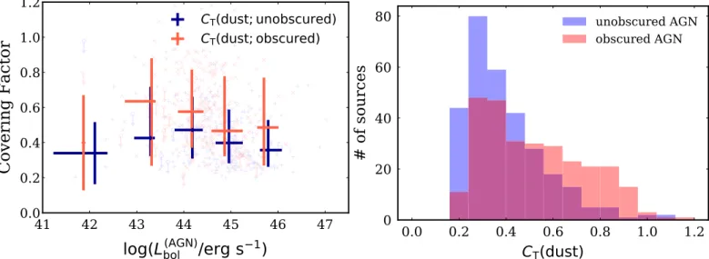
We compareC dustT( )between the AGN subgroups. The left panel of Figure10 showsC dustT( ) of unobscured(blue) and obscured (red) AGNs as a function of Lbol(AGN). Although the scatter is large, the binned C dustT( ) of obscured AGNs is always systematically higher than that of unobscured AGNs.
The right panel of Figure 10 shows the distribution of
( )
C dustT for unobscured(blue) and obscured (red) AGNs. The
( )
C dustT distribution for unobscured AGNs is clustered at
smaller values of áC dustT( )ñ = 0.41, while obscured AGNs are distributed over a widerC dustT( ) range, reachingC dustT( );
1.0. We apply the Kolmogorov–Smirnov (KS) test to these two samples: the p-value of the null hypothesis is 5.7×10⁻⁸and the KS statistic is 0.24, suggesting that the two distributions are Table 2
Equations of the Correlation in This Study
(1) (2) (3) (4) (5) Y X a b Reference m -⎛ ⎝ ⎜ ⎞ ⎠ ⎟ ( ) log L 10 erg s 12 mAGN 43 1
-(
)
log L 10 erg s 14 150 43 1 −0.24±0.03 1.08±0.03 Section4.3 -⎛ ⎝ ⎜ ⎞ ⎠ ⎟ ( ) log L 10 erg s MIRAGN 43 1-(
)
log L 10 erg s 14 150 43 1 −0.05±0.03 1.06±0.03 Section4.3 R log -⎛ ⎝ ⎜ ⎞ ⎠ ⎟ ( ) log L erg s bolAGN 1 4.52±1.25 −0.12±0.03 Section4.4Note.Correlation properties between two physical values. Columns:(1) Y variable; (2) X variable; (3) regression intercept (a) and its 1σ uncertainty; (4) slope (b) and its 1σ uncertainty; the equation is represented as Y=a+bX; (5) reference for the details of each equation.
Figure 7. R=LIR(AGN;1-1000 mm )/Lbol(AGN) as a function of the bolometric luminosity. The black crosses represent the median value of R in each bin of bolometric luminosity, with the error bars showing the inter-percentage range containing 68.2% of the sample.
significantly different, assuming that the significance level isα=0.05.
One possible origin of the difference is that the smaller
( )
C dustT for unobscured AGNs could be due to larger Lbol( ) AGN.
However, as discussed in Section 4.4.1, the luminosity depend-ence of C dustT( ) is unlikely, and the KS test shows that the distribution ofC dustT( ) for unobscured and obscured AGNs is
statistically significant even in each Lbol(AGN) bin for 42.5< <
-(L( ) )
log bol erg s 47
AGN 1 , with p-values of p<10−5 for
< (L( ) -)<
42.5 log bol erg s 45.5
AGN 1 and p=0.02 for 45.5<
<
-(L( ) )
log bol erg s 47
AGN 1 .
Another possible interpretation of the difference is as a consequence of the selection of unobscured and obscured AGNs. Several authors argue that AGN classification depends on the distribution ofC dustT( ); unobscured AGNs would be preferen-tially observed from AGNs with lowerC dustT( ), and obscured AGNs from AGNs with higherC dustT( ) (e.g., Ramos Almeida et al.2011; Elitzur2012; Ichikawa et al.2015; Lanz et al.2018).
5. Conclusions
We have constructed the IR(3–500 μm) SED for 587 nearby AGNs detected in the 70month Swift/BAT all-sky survey. Using this almost complete(587 out of 606; 94%) sample, we have decomposed the IR(3–500 μm) SEDs into SB and AGN components. The decomposition enabled us to estimate the AGN contribution to the 12μm (L12 m(AGNm )), MIR (LMIR(AGN)), and
total IR (LIR(AGN)) luminosities, as well as the contribution of
AGN luminosity to the 12μm (fAGN(12 mm )), MIR (fAGN(MIR)), and total
IR(fAGN(IR)) emission. Our results are summarized as follows.
1. The luminosity contribution of the AGN to the 12μm, MIR, and total IR band flux increases with the 14–150 keV luminosity. The AGN contributions to the 12μm, MIR, and total IR are almost 80%, 80%, and 50% at the high-luminosity end, respectively.
Figure 8.The covering factor(CT) as a function of the bolometric luminosity. The dust covering factors CT(dust) are obtained from R using the corrections reported in Stalevski et al.(2016). The covering factors of gas and dust CT(gas+dust) are obtained from the X-ray observations and the spectral fitting based on the obscured AGN fraction including Compton-thick AGNs(Ricci et al.2015,2017b). The Compton-thick fraction is fCT=0.32 forlog(Lbol(AGN) erg s-1)<43.5and fCT=0.21 forlog(L( ) erg s-)>43.5
bolAGN 1 . The orange crosses are shifted to the right by 0.1 dex for clarity.
Figure 9.The dust covering factor( (C dustT )) as a function of the bolometric luminosity. The simulated dust covering factorC dust; simT( )is obtained from the simulation using a random population following the L( )
IRAGN–L14–150 relation with a scatter of σ=0.4 dex (gray crosses) and σ=0.1 dex (pink crosses). The gray/pink crosses are shifted to the right by 0.1/0.2 dex for clarity.
2. We find nine pure IR-AGN whose IR emission is dominated by the AGN torus at least up to 90μm. These pure IR-AGN could be good candidates to create templates of the IR AGN SED, with an expanded range up to 90μm. Those sources could be easily selected using the color selection of f70μm/f160μm>1.0 and f22μm/f70μm>1.0. 3. Wefind a good luminosity correlation between the MIR
and ultrahard X-ray bands over five orders of magnitude (41<log(L14 150- erg s-1)<46). Our slope is almost consistent with that obtained by studies carried out using observations with high spatial resolution of nearby Seyfert galaxies, supporting our SED decomposition method, which would nicely estimate the intrinsic MIR emission without the contamination of star formation from the host galaxies.
4. Wefind that the average of the covering factor of gas and dust inferred from X-ray observations always exceeds the average of the covering factor of the dust torus, suggesting that the dust-free gas contributes to the absorption in X-rays. This gas could be located inside the dust sublimation radius, in agreement with previous observations based on X-ray occultation and spectral fitting studies of nearby AGNs.
5. The luminosity-dependent trend of C dustT( ) might originate from the large scatter of the luminosity correlations between LIR(AGN;1 1000 m- m ) and L14–150, and the trend would disappear once the scatter is removed. 6. Obscured AGNs tend to have larger C dustT( ) than
unobscured AGNs. This difference originates from the AGN classification, which depends on the distribution of the obscuring material.
We thank the anonymous referee for a careful reading of the manuscript and helpful suggestions that greatly strengthened the paper. We thank James Mullaney and Agnese Del Moro for providing the SB SED templates in this study, and Satoshi Takeshige for the technical discussion of IDL routine. We also thank Masatoshi Imanishi, Ryo Tazaki, and Daniel Asmus for
fruitful discussions. K.I. thanks the Department of Astronomy at Kyoto university, where a part of the research was conducted. This study benefited from financial support from the Grant-in-Aid for JSPS fellow for young researchers(P.D., K.I.), JSPS KAKENHI (18K13584; K.I.), and JST grant “Building of Consortia for the Development of Human Resources in Science and Technology” (K.I.). C.R. acknowl-edges the CONICYT+PAI Convocatoria Nacional subvencion a instalacion en la academia convocatoria año 2017 PAI77170080. F.E.B. acknowledges support from CONI-CYT-Chile (Basal-CATA PFB-06/2007, FONDECYT Reg-ular 1141218), the Ministry of Economy, Development, and Tourism’s Millennium Science Initiative through grant IC120009, awarded to The Millennium Institute of Astro-physics, MAS. K.O. is an International Research Fellow of the Japan Society for the Promotion of Science (JSPS) (ID: P17321). D.J.R. acknowledges the support of UK Science and Technology Facilities Council through grant code ST/ P000541/1.
Appendix A
Comparison with Studies from the Literature A.1. Comparison with the High-spatial-resolution Flux
Obtained with Ground-based 8 m Class Telescopes Here we compare the results in this study with the high-spatial-resolution observations by Asmus et al. (2014, 2015). Out of 122 high-spatial-resolution sources, we found 112 sources also used in this study. The remaining 10 sources were not found because they are located at low Galactic latitudes
<
∣ ∣b 10 , which we initially removed from the parent sample as discussed in Ichikawa et al.(2017).
The top left panel of Figure11shows the 12μm luminosity correlation between the high-spatial-resolution MIR observa-tions(L12 m(m );
Asmus Asmus et al. 2014,2015) and this study after
the SED decomposition(L12 m(AGNm )). The figure clearly shows that
our decomposition method successfully follows the one-to-one relation with the high-spatial-resolution observations down to Figure 10.Left: the dust covering factorC dustT( )of unobscured(blue) and obscured (red) AGNs as a function of the bolometric luminosity. Right: the distribution of
( )
m -
(L( ) )
log 12 m erg s 41.0
AGN 1 . The average of two parameters is
á L(m ) L(m )ñ =
log 12 m 0.05
Asmus 12 m
AGN . The standard deviation is
σ=0.36.
The top middle and top right panels of Figure11show the luminosity relation between L12 m(Asmusm ), L12 m(AGNm ), and the low-resolution 12μm luminosity before the SED decomposition
m
(L12 m(KI17)), which is taken from Ichikawa et al. (2017). Both panels show that the points are distributed equally to or below the one-to-one relations and suggest contamination of the host galaxy component inL12 m(KI17m ). The mean and standard deviation are álogL12 m(m ) L(m )ñ = -0.100.43
Asmus 12 m
KI17 . This shows that
the correlation betweenL12 m(Asmusm )andL12 m(AGNm )is tighter than that betweenL12 m(Asmusm )andL12 m(KI17m ), indicating that our decomposition method nicely reduces the contamination in the 12μm band from the host galaxies.
The bottom panels of Figure11show the same relations as those in the top panels, but for 12μm flux densities. All three panels also show a similar trend to the luminosity relations. One notable difference is that the flux density of the high-spatial-resolution observation (f12 m(Asmusm )) shows a decline in the
number of sources at around f12 m(Asmusm ) 10-2Jy. This is almost
consistent with the lower bound of theflux density observable with ground-based 8 m class telescopes with significant signal-to-noise ratio (Asmus et al.2014). Our study can explore flux
densities down to 10−3Jy, which is equivalent to the detection limit of the WISE W3 (12 μm) band. This is one of the advantages of the SED decomposition method using low-resolution, but sensitive space IR satellites compared to ground-based studies.
A.2. Comparison with Different Models from the Literature In this appendix we briefly compare the IR AGN luminosity obtained in this study and the ones obtained in Shimizu et al. (2017). They applied a different IR SED model to the IR data set, which is similar to ours but obtained from the Herschel observations in the Swift/BAT 58 month AGN catalog to study mainly the global star-forming properties in the host galaxies. Instead of using the AGN/host galaxy templates, they provided functions of the hot dust and the host galaxy respectively by following Casey(2012), and their functions are given by
n n n n = ⎛ -n n + ⎝ ⎜ ⎞⎠⎟ ( ) ( ) ( ) ( ) f Npl e S ,M ,T , 6 c MBB dust dust c 2
where the first term stands for the AGN component with the normalization Npland cut-off frequencyνc, and the second term
represents the host galaxy component of a single modified blackbody with a parameter of dust mass Mdust and a dust
temperature Tdust. Thefitting method used in their study is also
different from ours. They use a Bayesian framework with a Figure 11.Top: scatter plot of the 12μm luminosities obtained from high-spatial-resolution MIR observations (L(m );
12 mAsmus Asmus et al.2014,2015), this study after the SED decomposition(L(m )
12 mAGN), and before the SED decomposition (L12 m(KI17m );Ichikawa et al.2017). Blue crosses represent individual sources, and the orange dashed line represents the 1:1 relation. Panel show the luminosity relations betweenL12 m(Asmusm )andL12 m(AGNm )(left),L12 m(Asmusm )andL12 m(KI17m )(middle),L12 m(AGNm )andL12 m(KI17m )(right). Bottom: same plots as top but for 12μm flux densities.
Markov chain Monte Carlo procedure to obtain the posterior probability distribution function, and then use the median to obtain the best fitted parameters. Out of 307 sources in their sample, 204 sources have at least one Herschel detection and a reliable fitting quality (lir_agn_flag=0). After cross-matching with our sample, we found 180 sources in common. Again, the 24 sources removed are located at low Galactic latitude∣ ∣b <10 .
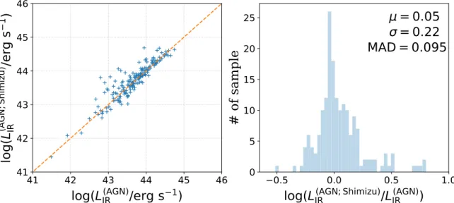
Since Shimizu et al.(2017) do not provide any 12 μm AGN flux or luminosity, we compare the total IR AGN luminosity obtained from their AGN component. The left panel of Figure 12 shows the correlation between the IR AGN luminosities obtained from Shimizu et al. (2017)
(L( )
IR
AGN;Shimizu) and the ones from this study. We find a good
luminosity correlation betweenLIR(AGN;Shimizu) and LIR(AGN). The Spearman’s rank coefficient is 0.91, and probability of the null hypothesis is P=4.9×10−69, suggesting that the correlation is significant. The average of the distribution of r=
(L( ) L( ))
log IR
AGN;Shimizu IR
AGN is also shown in the right panel of
Figure 12. We do not find any systematic offset between the two methods (μ=0.05) with a standard deviation of σ=0.22 dex. Since there are several outliers with
>
(L( ) L( ))
log IR 0.3
AGN;Shimizu IR
AGN , we also compute the median
absolute deviation(MAD) and the value is MAD=0.095 dex, which is smaller than the standard deviation by a factor of two. As already mentioned in Shimizu et al. (2017), their model
allows the power-law component to extend to longer wavelengths, which would return slightly larger AGN luminosities with log(LIR( ) L( ))>0.3
AGN;Shimizu IR
AGN for some
cases. Those sources are actually seen in Figure12but they are only a small percentage of the sample. Thus, we conclude that, although the fitting methods and the template are different, each model returns the consensus results for the estimation of the IR AGN luminosities.
Appendix B
Flux Correlation between 12μm, MIR, and 14–150 keV Bands
Figure 13 shows the flux correlation between the AGN 12μm, MIR, and 14–150 keV bands, revealing a clear correlation between the bands even in the flux–flux plane. The Spearman’s rank coefficient is 0.43 and the probability of the null hypothetical is P=10-28 for both flux–flux
correla-tions, suggesting that the correlation is significant. The slopes are b=1.48 for the AGN 12 μm band and b=1.49 for the AGN MIR band, respectively. As we discussed in Ichikawa et al.(2017), there is a clear decline in the number of sources at
<
-
-f14 150 10 11erg s−1cm−2, while MIRflux can go down to 3×10⁻¹³erg s−1cm−2, which is the typical detection limit of the MIR band. This trend suggests that the sample is limited by the detection limit of the X-rayflux.
Figure 12.Left: scatter plot of total IR AGN luminosities obtained from Shimizu et al.(2017) (L( )
IRAGN;Shimizu) and those obtained from this study (LIR(AGN)). Blue crosses represent individual sources, and the orange dashed line represents the 1:1 relation. Right: histogram ofr=log(LIR(AGN;Shimizu) LIR(AGN)). The meanμ, standard deviationσ, and median absolute deviation (MAD) of r are also shown.
Appendix C
Comparison of Relation between CT andLbol( ) AGN
using Different Values
C.1.C dustT( )Estimated from the Observed 12μm Luminosity It is important to check whether the same result in Figure8is obtained using the MIRfluxes without host galaxy subtraction. To achieve this, we estimate the total IR AGN luminosity by assuming that the observed 12μm luminosity originates from the AGN emission. Then we use the conversion factor of
m
-( )
LIRAGN;1 1000 m/L12 m(AGNm )=2.77 estimated from the AGN
template in this study. The calculation of R and then
( )
C dustT is performed in the same manner as we discussed in
Section 4.4. The left panel of Figure 14 shows the relation between CT and Lbol( )
AGN using
( )
C dustT estimated above. It
clearly shows that while the resultC dustT( )<C gasT( +dust)
holds for43.5<logLbol( )<45.5
AGN ,
( )
C dustT becomes almost
equal to C gasT( +dust) in the luminosity bin 42.5< <
( )
L
log bol 43.5
AGN , which is not seen in Figure 8. We also
apply the KS test between C dustT( ) and C gasT( +dust) for
eachLbol(AGN)luminosity bin. In order to apply this test, we make a Gaussian distribution ofC gasT( +dust)in which the central value is the average ofC gasT( +dust)and 1σ is its standard deviation, and the number of sources is the same as for
( )
C dustT in the same Lbol( )
AGN bin. As a result, we find a
significant difference for the luminosity bins with < L( )<
43.5 log bol 45.5
AGN with p-values of p<10−30, while
the clear significance is not obtained for the luminosity bins < ( ) L log bol 43.5 AGN (p>0.5) and < L( ) 45.5 log bol AGN (p=
0.26). This difference originates from the flux subtraction after the SED decomposition, especially at the lower AGN luminosity end, suggesting its importance and its effect on estimating the dust covering factor.
C.2. Dependence of the Bolometric Corrections Here we summarize whether different bolometric corrections can affect the relation shown in Figure 8. In this study, following the method used in Ricci et al. (2017a), we use a constant bolometric correction of Lbol(AGN)/L14–150=8.47,
which is based on Lbol(AGN)/L2–10=20 under the assumption
ofΓ=1.8, the median value of the Swift/BAT 70 month AGN
sample(Ricci et al.2017b). On the other hand, Marconi et al. (2004) account for variations in AGN SEDs to obtain the bolometric correction with AGN luminosity. They assume a varying relation between optical/UV and X-ray luminosity, which is called a luminosity-dependent bolometric correction. This gives a larger bolometric correction than the constant one at the higher AGN luminosity end, which would make average
( )
LbolAGN larger and CTsmaller.
The right panel of Figure14shows the same plot as Figure8, but using the luminosity-dependent bolometric correction of Marconi et al.(2004). As expected from the luminosity-dependent bolometric correction, the distribution is slightly shifted to the right and downward in the figure. Actually, the median values of AGN bolometric luminosity and C dustT( ) change from(logLbol(AGN),CT(dust))=(44.65, 0.46)to(logLbol( ), AGN;M04
=
( )) ( )
C dustT 44.79, 0.39.
The figure clearly retains the trend of C gasT( +dust)
( )
C dustT over the entire AGN luminosity range. On the other
hand, the slight decline in C dustT( ) in the lowest AGN bolometric luminosity bin disappears in Figure 14. This is mainly because of the small statistics in the lowest luminosity bin and some sources being shifted into a higher luminosity bin because of the larger bolometric correction by Marconi et al. (2004).
C.3. Dependence of Additional Torus Parameters We here discuss how the dust covering factor changes when we change the set of the torus parameters. In this study we have only considered the spectral power-law index(α1) at λ<19 μm
for the high-luminosity end with logL14 150- >44, and not
considered the dust extinction for obscured AGNs, which could be one of the most significant parameters shaping the torus SEDs. The left panel of Figure 15 showsC dustT( ) as a function of
( )
LbolAGN after addition of the dust extinction for obscured AGNs using the absorption profile of Draine (2003) (see also Mullaney et al. 2011). C dustT( ) becomes slightly larger, but the overall sense does not change. The middle panel shows the same plot using afixed power-law index α1=1.8 for all sources without
the dust extinction. C dustT( ) shows a flatter distribution than Figure 8, but the overall trend ofC dustT( )<C gasT( +dust)
still holds.