A Large-Scale Marketing Model using
Variational Bayes Inference for Sparse
Transaction Data
著者
Ishigaki Tsukasa, Terui Nobuhiko, Sato
Tadahiko, Allenby Greg M.
journal or
publication title
TMARG Discussion Papers
number
114
year
2014-01
TOHOKU MANAGEMENT
&ACCOUNTING RESEARCH GROUP
Discussion Paper No. 114A Large-Scale Marketing Model using Variational Bayes Inference for Sparse Transaction Data
Tsukasa Ishigaki Nobuhiko Terui
Tadahiko Sato Greg M. Allenby January , 2014
GRADUATE SCHOOL OF ECONOMICS AND MANAGEMENT TOHOKU UNIVERSITY KAWAUCHI, AOBA-KU, SENDAI 980-8576 JAPAN
1
A Large-Scale Marketing Model using Variational Bayes Inference for Sparse Transaction Data
Tsukasa Ishigaki* Nobuhiko Terui* Tadahiko Sato** Greg M. Allenby***
January, 2014
*Graduate School of Economics and Management, Tohoku University, Sendai 980-8576, Japan ** Graduate School of Business Science, University of Tsukuba, Tokyo 112-0012, Japan *** Fisher College of Business, Ohio State University, Columbus, OH, U.S.A.
Ishigaki acknowledges the financial support of KAKENHI Grant-in-Aid for Young Scientists (A) 24683012. Terui acknowledges the financial support of the Japanese Ministry of Education Scientific Research Grants (A) 25245054.
2
Abstract
Large-scale databases in marketing track multiple consumers across multiple product categories. A challenge in modeling these data is the resulting size of the data matrix, which often has thousands of consumers and thousands of choice alternatives with prices and merchandising variables changing over time. We develop a heterogeneous topic model for these data, and employ variational Bayes techniques for estimation that are shown to be accurate in a Monte Carlo simulation study. We find the model to be highly scalable and useful for identifying effective marketing variables for different consumers, and for predicting the choices of infrequent purchasers.
Key words and phrases:
database marketing, dimension reduction, Bayesian analysis, choice models, topic model, targeting
3
1. Introduction
Modern analytic techniques in marketing are continuously confronted with the necessity of extracting relevant information from large volumes of data by identifying important drivers of consumer behavior. It is common for datasets to record household purchases of products that are orders of magnitude larger than what current models of behavior are currently capable. Existing models of choice and demand, for example, are typically limited to less than twenty or so product alternatives that are tracked across possibly hundreds of consumers (see Rossi et al. 2005 and Chintagunta and Nair 2011).
Increasing the number of products analyzed is problematic because of potential complexities in the structure of demand and the accompanying increase in the required number of model parameters. Increasing the number of respondents is also problematic because of computational constraints arising from respondent heterogeneity that is found to be important in describing demand and deriving policy implications. While a variety of dimension-reducing techniques have been studied in the fields of statistics and data-mining, the presence of heterogeneous consumers and heterogeneous purchase environments with prices and other variables change over occasions requires the use of model-based inference as opposed to methods applied directly to the marginal data (Chintagunta and Nair 2011).
Naik et al. (2008) discusses three solutions to the challenges in massive data analysis: increasing computer power, employing alternative approaches for data analysis, and using scalable estimation methods. In this paper, we combine the second and third options to obtain improved inferences about consumer behavior in large datasets. We extend the voting bloc model of Spirling and Quinn (2010) and Grimmer (2011) that are a variation of topic models used to conduct large-scale analysis of text data (Blei et al. 2003).
The topic model is a generalization of a finite mixture model (Kamakura and Russell 1989) in which each data point is associated with a draw from a mixing distribution (Teh and Jordon 2010). Models of voting blocs (Spirling and Quinn 2010), for example, track the votes of legislators (aye or nay) across multiple bills, with each bill associated with a potentially different concern or issue. Similarly, the latent Dirichlet allocation (LDA) model of Blei et al. (2003) allocates words within documents to a small number of latent topics whose patterns are meaningful and interpretable. Each vote and each word is associated with a potentially different issue or topic, and hence the mixing distribution is applied to the individual datum. In our
4
analysis of household purchases, we allow every purchase (and every non-purchase) in every product category to be related to a potentially different latent context (topic, or issue) for which the good is purchased. This allows us to view a consumer's purchases as responding to different needs or occasions (e.g., family dinner, snacks, etc.), and allows us to identify the ensemble of goods that collectively define latent product segments across a large number of products.
We obtain a scalable estimation method by employing variational Bayes (VB) inference as in Jordan et al. (1999) and Bishop (2006), instead of the standard Markov chain Monte Carlo (MCMC) inference. MCMC methods can incur large computational cost in large-scale problems. VB inference approximates a posterior distribution of target by variational optimization in a computationally efficient manner.
Our approach combines variational Bayes (VB) methods, as in Jordan et al. (1999) and Bishop (2006), with a topic-like probit model to obtain a computationally feasible model of consumer purchases that is scalable to large databases. Individual-level inference is possible in our model, where we can identify the marketing variables that are effective for specific individuals and the products for which they are effective. Our model is therefore similar to adaptive personalization systems proposed by Ansari and Mela (2003), Rust and Chung (2006), Chung et al. (2009) and Braun and McAuliffe (2010). However, it is different in that our model structure facilitates analysis of a much larger array of product categories.
In the next section, we propose a model for consumer purchases in multiple product categories. Section 3 describes a variational Bayes inference scheme for the models and a simulation study that verifies the scalability. The prediction performance of the proposed models is presented in Section 4. Section 5 applies the model to actual customer purchases in a general merchandise store. Discussion and concluding remarks are presented in Section 6.
2. Model
Estimating parameters of choice model for a large number of consumers and products is often computationally infeasible. In addition, the actual sample size of transactional data is often much smaller than the data space reflected by a data cube with dimensions corresponding to the number of consumers, number of products and time, making fixed-effect estimates of model parameters with heterogeneity unsuitable. We address this challenge by relating consumer purchases to latent segments (similar to topics and blocs) that greatly reduces the
5
dimensionality of the model. Response parameters are then introduced in the reduced dimensional space by connecting each choice to marketing variables with a hierarchical probit model.
2.1 Dimensional Reduction by Topic Models
Dimensional reduction is an important technique in massive data analysis. Here we briefly introduce the idea of introducing a latent variable to common in topic models in the context of consumer purchases. We seek the probability p i c
| that consumer c purchases item i . Dataset includes C consumers and I product items through T periods. However, the probabilities cannot be directly calculated because of computational difficulty imposed by the large-scale setting and data sparseness. The topic model calculates p i c
| by introducing a latent class z
1, ,Z
whose dimension is significantly smaller than the number of consumers and items (ZC I, ).The latent variable is used to represent the sparse data matrix as a finite mixture of vectors commonly found in topic models:
1 ( 1 | 1) ( 1 | ) (1 | ) ( | 1) ( | ) . ( | 1) ( | ) ( | )
Z z p i c p i c C p z p z p z C p i I c p i I c C p I z (1)More specifically, we decompose a large probability matrix of size CI to two small probability matrices of sizes I and Z ZC based on the property of conditional independence.
The main difference between voting blocs model and LDA is assumed distributions for probabilities p i z
|
in the I size probability matrix. The voting blocs model Zsupposes a Bernoulli distribution for the probability p i z
| . LDA assumes a categorical distribution for the probability matrix.In the analysis of purchase behavior using topic models for large consumer transaction data, Iwata et al. (2009) extracted dynamic patterns between purchased product items and consumer interests. Ishigaki et al. (2010) fused heterogeneous transaction data and consumer lifestyle questionnaire data, while Iwata et al. (2012) identified consumer purchase patterns by using a topic model with price information on the purchased products. These approaches identify patterns among consumers and product items. The labeled LDA proposed by Ramage et al. (2009), and the supervised LDA of Blei and McAuliffe (2007) extend the topic models
6
by incorporating additional data in the analysis. However, none of these approaches are suitable for relating marketing variables to individual consumer choices as explanation variables. In the following sections, we construct a model that links marketing variables with consumers and products.
2.2 A Reduced Dimensional Choice Model
Let ycit denote consumer c’s purchase record of product i at time t, assigning ycit 1 if consumer c purchased the item, and ycit 0 otherwise. Denote ucit as the utility of consumer c’s purchase record of product i at time t. We assume a binary probit model with
0
cit
u if ycit 1, and ucit 0 if ycit0. We couple the topic model in (1) with the binary choice probability as in a voting bloc model to obtain the choice probability:
1
( cit 0)
Zz ( cit 0 | ) ( | )p u p u z p z c . (2)
We denote the utility associated with the latent class z as ucit( )z , and then the choice probability can be represented as p u
cit 0 |z
p u
cit( )z 0
. Assuming a linear Gaussian structure on the segment utility ucit( )z with marketing variables as
( )
,1
z T
cit it zi
u N x β , the right hand side of (1) is represented as,
1 1 1 ( ) ( |1) ( | ) ( ) T t z Z z T It zI F p z p z C F
x β x β (3)where βzi
zi1,,ziM
Tis a response coefficient vector of latent class z with respect to itemi, xit
xit1,,xitM
T is a vector of M marketing variable for item i at time t, and F
is the cumulative distribution function (CDF) of the standard normal distribution. In our empirical study, xit includes price and promotional variables.We next set a categorical distribution Ccz for the probability p(z|c) that consumer
c belongs to the latent class z. The categorical distribution is multinomial with parametersC . c
The C is determined so that the selection probability of consumer c with respect to item i is c
conditionally independent if the latent class z is given. Then, the right hand side of (1) is
represented by:
1 1 1 1 ( ) ( ) T t z Z z Cz z T It zI F C C F
x β x β (4)7
Finally, segment-level heterogeneity is introduced through a hierarchical model with a random effect for response coefficient βzi
,
zi NM i Vi
β μ , (5)
where the prior distributions for μi and V follow an M-dimensional multivariable normal i
distribution NM
μ ,Vi
and an inverse-Wishart distribution IW
W w , respectively. ,
μ ,
, W andw
are hyperparameters. That is, we assume that the M-dimensional coefficient vector
zi for each segment, z, is a draw from a distribution with mean and covariance that is item-specific.We specify a prior distribution for C , assuming the Dirichlet distribution as the c natural conjugate prior distribution of categorical distribution:
~ Dirichlet
c
C γ , (6)
where γ is a hyperparameter vector of the Dirichlet distribution. The likelihood is given as
1 1 { } |{ },{ },{ } | , , , c c C Z cit c zi it cz cit it zi c i I t T z l y C p y z
C β x x β (7)where p y
cit |x βit, zi,z
denotes the kernel of the binary probit model conditional on z, Tcdenotes a subset of t in which consumer c purchased any item in a store, and Ic is a subset of items i purchased by consumer c during the period t 1, ,T , that is,
| 1 0
I c i cit T t
y and
1 | T 0 c t cit I i
y .Equation (7) is difficult to use directly because the likelihood includes summations over latent class z. Instead, we employ a data augmentation approach by Tanner (1987) with respect to latent variable z. We introduce variables zcit
1, ,Z
denoting the label of thelatent class for each consumer c, each purchased item i, and each purchasing event t. Conditioning on the zcit for each purchasing transaction, as in the LDA of Blei et al. (2003), the likelihood in (7) simplifies to:
1
{ } |{ },{ },{ },{ } | | , ,
c c
C
cit c cit zi it cit c cit it zi cit c i I t T
l y z p z p y z
C β x C x β , (8)
where p z
cit |Cc
denotes a categorical distribution when C is given. cOur model for massive data analysis is different to the LDA model in that it only deals with the presence of products appearing in the purchase basket of the consumer, and does not deal
8
with non-purchase of product. This is different to model encountered in the analysis of text data where it is the presence of words, and not their absence, that characterizes the latent topics. The co-occurrence of the products selected during a shopping trip is what gives meaning to segments, as modified by the marketing variables.
The posterior distribution of parameters including latent variables {zcit},{ucit( )z} is then given by
( ) ( ) ( ) ( ) { },{ },{ },{ },{ },{ } | { },{ } | { } | , , , | , , , , | { } | , , , { },{ },{ },{ },{ },{ },{ },{ } = zc cit cit zi i i it cit c cit
cit c zi it cit z
cit zi cit it cit i i zi
z
zi cit i i it z
c cit cit zi i i it cit
p z u V y p z p z y p u z y p V p u V p z u V y C β μ x C C β x β x μ β β μ x C β μ x
1 1 1 ( ) 1 , | , | | , , ,
c c C I Z c i i zi i i c i z C zcit c cit cit zi cit it c i I t T p p V p V p z p y u z C μ β μ C β x (9)
3. Variational Bayes Inference
We introduce VB inference in order to achieve computational feasibility for large-scale transaction data. VB inference approximates the posterior, or target distribution in a Bayesian model. The advantage of this method over MCMC is low computational cost. VB also takes advantage of parameters that can be decomposed into several mutually independent groups. This is necessary for our analysis using a large database.
The target and approximate distributions are denoted as p and q, respectively. The latter is called the variational distribution. Distributions p and q share a parameter set
θ
. In general, when the data D is given, the log marginal likelihood p D of the target distribution is ( ) decomposed into two components as9
1 1 log ( ) ( ) ( || ), ( ) ( ) log ( , ) ( ) , KL( || ) ( ) log ( | ) ( ) . p L q KL q p L q q p q dZ q p q p q dZ
D θ D θ θ θ θ D θ (10) ( )L q is called the variational lower bound in VB inference, and KL( || )q p is the
Kullback–Leibler divergence of the target and variational distributions. As is well known, KL( || )q p is zero if p and q are the same distribution. Therefore, a reasonable solution to
estimating the posterior distribution p is the variational distribution q for which KL( || )q p is
minimized. However, it is difficult to evaluate the value of KL( || )q p because the expression
involves a posterior distribution of ( | )p θ D .
In contrast, L q involves a joint distribution ( ) p D θ that is easily evaluated in many ( , ) cases because it is obtained as the product of the prior and the likelihood in Bayesian models. We note that maximizing ( )L q is equivalent to minimizing KL( || )q p because the log
marginal likelihood of the target distribution is constant for a given dataset. In this situation, assuming that the distribution q and parameter set
θ
are decomposable for some groups as
J
( )*j j jq θ
q θ , where the parameters θ are called variational parameters, ( )( )*j L qcan be maximized by the following updating algorithm (Jordan et al., 1999):
( )* ( )*{ } ( )* arg max exp log , . j J j new j j j i j L q p
θ θ θ E D θ (11)The Ei j
are the expectation value associated with q distributions over all parametersj( )*j
θ , where i j . The variational parameters are updated for each variational parameter set
( )*j
θ
until convergence of the algorithm. The initial variational parameters are proper random values. The VB is guaranteed to converge after several iterations because L q is convex with ( ) respect to each q θj
( )*j (Bishop, 2006). The variational lower bound monotonicallyincreases as the iteration proceeds; therefore, convergence can be confirmed by checking the value of L q at each iteration. ( )
3.1 VB for the Proposed Model
We introduce the variational distributions and parameters for the modes of proposed model. The parameters and variational parameters are denoted as
( )
{ },{ },{ },{ },{ },{ }
z
c zcit ucit zi i Vi
10
* * * ( )* * * * * * * , , , , , , , , z cit c cit iz Viz i i wi Wiθ C γ β μ μ respectively, while the
variational distributions are configured as
* * * ( ) ( )* 1 1 1 * * * * * * , 1 1 1 | ,{ },{ } | | | , , | , , | , , ,
c c c c it cit C C C z zc c c z cit cit u cit cit it cit
c c i I t T c i I t T I Z I zi zi zi V i i i i i i i z i q y q q z q u z q V q V w W θ θ x C γ C β x β μ μ μ (12)
where
q
c is a Dirichlet distribution with variational parameter γ*c,q
c is a categorical distribution with variational parameter C*cit ,q
u is a truncated normal distribution with parameterz
cit and variational parameter β( )*citz , q is an M-dimensional multivariable normal distribution with two variational parameters (mean vector μ*zi and covariance matrix*
zi
V ), and q V, is a multivariable normal–inverse Wishart distribution with variational
parameters μi*,
i*,w Wi*, i*. Here, to realize effective variational inference, we assume that all variational parameters are independent. The update equation and the derivations of the variational parameters are detailed in Appendix A.4. Simulation Study
In this section we examine the performance of the proposed VB estimator relative to MCMC using simulated data. We show that MCMC becomes too computationally demanding as the size of the dataset increases, and that VB provides a computationally efficient and accurate approximation to the posterior with good predictive properties.
The simulation datasets are generated as follows:
a) We determine the number of consumers, items and time period for the dataset. b) Consumers randomly are assigned to a segment. Consumers assigned to same
segment have a same product set of items, which are a subset of items that consumers evaluate when making a purchase decision. The number of consumer segments and the number of items in a product set is set to 0.02 C and 0.2 I , respectively, where
C and I are varied in our analysis.
c) Items in a product set are randomly assigned from all available items, with a lower bounds on the number of items needed in the set.
11
d) The marketing variables are comprised of xit
1,Pi T, where Pi is a price discount rate generated from a uniform distribution with interval [0.1 1.0].e) Each consumer randomly visits the simulated shop on five occasions during data period T, and purchases N items with probability proportional to the discount from production set.
Computational time and predictive results are calculated using data simulated from the above steps. The computational results reported below were calculated in same computational environment (64-bit version of Python 2.7.5, implemented on a 3.5 GHz processor (Quad-Core Xeon; Intel Corp.) with 64 GB memory).
4.1 Scalability
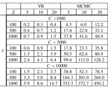
The scalability is investigated under the condition as follows: C = {1000, 5000, 10000}, I = {100, 500, 1000}, T = 30, Z = {5, 10, 20} and N = 10. Thus, 27 different scenarios were explored in the simulation study. The simulation times in hours are shown in Table 1. Here, we set hyperparameters as γ
0.1,, 0.1
T , μ
0,, 0
T , 1, W IM, w 10 inVB and MCMC. I means identity matrix of size M M. In VB method, iterations are terminated when the variational lower bound improves by less than 5
10 % of current value in two consecutive iterations. The MCMC method uses Gibbs sampler, and its simulation times of 6,000 MCMC samples are estimated from those of 10 samples, as is to be computationally infeasible. We also note that the selection of 6,000 MCMC samples is consistent with the simulation study of Braun and Mcauliffe (2010). Three kinds of settings for hyperparameters, stopping rule of VB iteration and the number of MCMC samples, defined above, are adopted in all empirical studies hereafter.
Table 1 shows the computational time for VB and MCMC methods. In both algorithms, the cost increases approximately linearly with the size of the dataset specified in term of the number of consumers, items, and latent classes. In all scenarios, the computational time of MCMC exceeds that of VB. The VB algorithm is around 20 to 50 times more efficient than MCMC, depending on the scenario. The time of estimation using large-scale data (C = 10000,
I = 1000) by MCMC is estimated over 450 h, and thus we recognize that MCMC is not
12
Table 1 : Simulation time by VB and MCMC
4.2 Data Sparseness and RMSE of Prediction
The predictive performance of the models is investigated by simulation, focusing on whether the model can adapt to sparse data or not. Sparse data are commonly encountered in datasets containing many items. In this paper, we define the data density rate (DDR) as
1 1 1 1
C I T cit c i t DDR C I T y (13)The DDR specifies the rate of ycit events in the data space. The N controls values of DDR 1 in the simulation dataset. Here we generated datasets for C = 500, I = 100, T = 100, Z = 20, and
N = {2, 4, 6, 8, 10}; this specification of N implies that DDR = {0.1%, 0.2%, 0.3%, 0.4%,
0.5%}. DDRs of actual scan-panel datasets are, to our knowledge, always below 1 %. The prediction performance is measured by the root mean square error (RMSE), given by
1 2 1 1 1 ( 1) c C C I c cit cit c c i t T RSME I T y p y
(14)where Tc denotes the number of elements T for each consumer; that is, the number of store c
visits within the specified data period. The
p y
(
cit
1)
is calculated by1 ( )
Z T
cz it zi z C F
x β .The hold-out and hold-in samples are generated by the same procedure. Using the Gibbs sampler, we generate 6,000 samples of each parameter, where the first 5,000 are discarded as burn-in samples.
Table 2 shows the average RMSE obtained in three simulation trials of DDR for each of four methods, namely Random, Homogeneous, VB and MCMC. In this simulation, we set five levels of DDR from 0.1% to 0.5%. “Random” means the situation that consumers are permitted completely random choice of purchased items and shop visits, and its RMSE is approximately 0.577. “Homogeneous” implies the model with Z = 1. We first observe that the proposed models works well compared to “Random”. Second, heterogeneity significantly improves the predictive performance. Third, the performances of VB and MCMC are comparable. These properties hold throughout every setting of DDRs.
13
5 Empirical Application Using Customer Database
In this section, we apply the proposed model to a real large-scale customer dataset. The results of the simulation study indicate that the VB estimator provides a close approximation to the MCMC with a large improvement in computational speed. We use VB in the empirical application in this section and report on estimation results and their managerial implications.
5.1 Data and Variables
A customer database from a general merchandise store, recorded from April 1 to June 30 in 2002, is used in our analysis. A customer identifier, price, display, and feature were recorded for a given purchase occasion. The dataset contains 162,775 transactions involving 1,647 consumers and 1,004 items. The 1,004 selected items were displayed or featured at least once in the data period. The DDR of the scan-panel data is 0.31 %.
The marketing variables are price (Pit ), display (Dit), and feature (Fit ); that is,
1
Tit Pit Dit Fit
x . Pit is the price relative to the maximum price of item i in the observational period. Display and feature are binary entries, equal to one if the item i is displayed or featured at time t, and zero otherwise.
5.2 Model Comparisons
The proposed models are compared in terms of RMSE. The parameters are estimated with the number of segment Z = {2, 3, 4, 5, 10, 20}. The hold-out sample comprises records from July 1 to September 30, 2002. The RMSEs for comparable models are shown in Table 3. We observe that our proposed models (Z greater than two) have smaller value of RMSEs than “Random” and “Homogeneous” models. The models with Z greater than five have the same RMSEs and thus we understand that the model with Z = 5 is appropriate for the empirical analysis below.
The comparison of RMSE of (i) all customers with that of (ii) infrequent customers provides useful information of the performance of our models. The largest number of purchases by one customer in our data is 390 items and 88 visits to the store, and we define infrequent customers as those with fewer than five purchases and three visits to the store. The predictive performance of infrequent consumers slightly decreases compared to that of all consumers,
14
however, the RMSE is almost equivalent to that all customers. Thus, our models present a tolerable prediction performance for even infrequent consumers.
Table 3 : RMSEs for real customer database – all and infrequent customers
5.3 Segment-Level Parameter Estimates
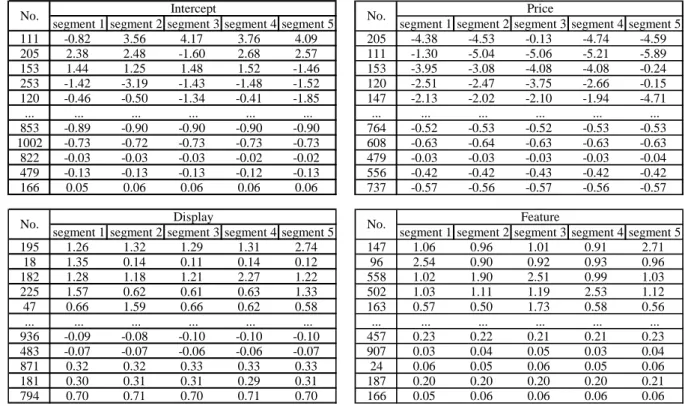
Table 4 displays the parameter estimates for “Price”, “Display” and “Feature” and “Intercept.” The rows of the tables correspond to products, and the columns to the segments. The rows are ordered in terms of the differences of estimates among the segments. The first row of each table is for the product estimates with maximum variation, and the last row of each table corresponds to estimates with minimum variation. The products positioned near the top of the table have larger heterogeneity in the response parameters, while those at bottom of the table have relatively similar values among segments. The products are identified in terms of their sales rank, with the product named “No. 1” the most purchased product in our database. We observe that “Price” coefficients are estimated negative and “Display” and “Feature” are positive for most products. This means that our proposed model produces economically reasonable estimates. The coefficient estimates also indicate the effectiveness of the marketing mix variables for each product. In the “Price” table, for example, product No. 205 has the highest rank and consumers in segment 3 do not respond to variation in price for this product. For product No. 111, segment 1 is the least price sensitive and for product No. 153 the price insensitive segment is segment 5. Similar results are found with the display and feature portions of the table, where we see that the most responsive segment is product-specific. We also find that the lower ranked products in each table show nearly uniform response in each segment. The results imply that marketers can perform effective promotions to specific segment for higher ranked products, however, homogeneous promotions to any segments are enough for lower ranked products.
Table 4: Characteristics of βzifor the five segments of consumers
Next, we extract relative preferences of product category for five segments. First, we define the relative preference score of segment z for product i by using estimated intercepts for
15 product i as 1 0 1 0
Z zi zi z ziRP Z . The consumers in segment z with the highest value of
zi
RP relatively prefer product i than consumers in other four segments. Thus, we observe
preference of five segments by ordering of the score with respect to each segment.
For visualization of segment’s preferences, we count the number of product category in top 100 products in order of RP with respect to each segment. Table 5 shows name and zi
number of product categories containing over three kinds of products in the top 100 products for each segment. It discloses consumer’s preferences of purchased products for estimated segments.
Table 5: Relative preferences of purchased product category for five segments
5.4 Individual Level Parameter Estimates
Individual level estimates of market response is obtained by taking expectation of segment level estimates with respect to Ccz
1
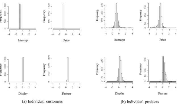
Z ci cz zi z C α β . (15)We characterize individual consumer in terms of her estimated response coefficient αci. The empirical marginal distribution of individual consumer parameter estimates taking average
1
1 1, , I ci i i I I
α of 1,647 products for each marketing variable are displayed by histograms in Figure 1(a). On the other hand, the empirical marginal distributions of individual product, taking average over 1004 consumers, i.e., of
1 1
1, , C ci c c C C
α , are depicted in Figure 1(b). The products that never displayed and featured in the data period have been omitted.The marginal distributions provide reasonable individual consumer estimates since almost intercept’s and price’s coefficients are negative and almost display’s and feature’s coefficient are positive. The distributions of individual product estimates show that the feature’s distribution has a sharp peak around zero, implying that promotions by display and feature are effective for many products, however, there are a lot of products that they are not
16
effective for the feature.
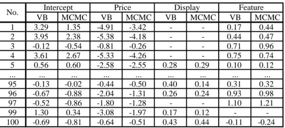
Table 6 shows the results of testing the significance of estimated response coefficients for individual consumers and products by using the 95% HPD (highest probability density) region. Owing to the space constraints, the results are shown for a portion of the dataset (five consumers and five products). “*” signifies that the 95% HPD region does not contain zero; if the HPD region includes zero (i.e., if the coefficient is insignificant), this square is left blank. We call this graph “Customer-Promotion Diagram”. For example, in the “Price” diagram, the purchase of No.253 by consumers (a) and (b) is highly influenced by price; however, the price of No. 318 affects the purchasing behavior of consumers (a) only. We also report that discounting No.18 will not promote consumer (b) to purchase it. This analysis informs retailers and marketers which promotion of specified product is effective to any specific individual consumer. Thus, our proposed model enables marketers to develop effective pricing and promotional strategies for targeted consumers and products.
Table 6: Personalized effective marketing variables for individual consumers and products
Figure 1 Marginal distribution of parameter estimates of individual consumers and products
5.5 Precision of Approximation to Posterior Density
We examine the precision of VB by comparing estimates to those obtained with MCMC, as is assumed that MCMC is a more correct than VB as long as there are sufficient iterations to fully characterize the posterior distribution. For comparison purposes, we reduced the size of data so that MCMC computations terminate within one day. We extracted 500 customers randomly from our dataset, and choose the top 100 products in terms of sales volume. Table 7 shows estimates of response parameters for VB methods. The vector of estimates for 100 products are displayed in row according to the order of number of purchases, that is, first row specifies the estimates for the most purchased product. The numbers in the table are sample mean of segment level estimates. “-” mean the product which has never displayed or featured in the record. From this result, we observe that price coefficients are reasonably estimated in the sense most of product have negative values. The same thing holds for the coefficients of display and features. That is, our proposed models perform well.
17
Table 7 : Estimated parameters by VB and MCMC
6. Discussion
This paper addresses two challenges in estimating models of demand in large databases: i) the large number of available products and ii) the large number of consumers who purchase these products. Existing models in marketing and methods of estimation tend to focus on a narrow set of products and a subset of consumers to understand the richness of the competitive environment within a product category among a random sample of consumers. This goal, however, is often at odds with the goals of practitioners who want to score existing datasets to identify a wide set of customers and products to allocate promotional budgets and increase sales.
We propose a descriptive model of demand based on the idea of topic models where products purchased by consumers take the place of words used by authors in creating documents. We allow for a product's purchase probability to be affected by price, display and feature advertising variables, but do not treat purchases to arise from a process of constrained utility maximization. The advantage of this approach is that it allows us to side-step complications associated with competitive effects and model a much larger set of products than that possible with existing economic models. By retaining prices and other marketing variables in our model we can still predict the effect of these variables on own-sales. This tradeoff is inevitable in the analysis of large-scale databases where purchases are tracked across thousands of products. The proposed model links the characteristics of consumer segments to marketing variables, and it is applicable to both segment-level and individual-level marketing across a large set of products.
The scalability and predictive performance of the proposed models were confirmed through a simulation study involving variational Bayes inference. In our analysis, we imposed a fairly conservative convergence criteria for VB of 105%, but also found that coarser thresholds (for instance, 103%) produced similar results. We therefore believe that estimation times can be further reduced in practice from those reported in this paper.
Finally, we employed the RMSE criterion for choosing the number of segments. In the VB framework, the variational lower bound is used for this criterion, as is shown in, for
18
example, Corduneanu and Bishop (2001). The variational lower bound in our models is somewhat sensitive to changes in the number of segments, Z. We identify this as a future research.
19
Appendix A: Derivation of VB Algorithm for Proposed Model
This appendix details the variational inference of proposed model. The update procedure derives from the analytical calculation of equation (13). The update equation for each
variational parameter is obtained from the following expectation values
( )* ( )* log , log , log , ,
j q i j i i i i j p p p q d E D θ E D θ D θ θ θ (A1) where D
xit , ycit
.The update procedures of variational parameters Ccit* , γ*c, β( )*citz , μ*iz, Viz*, μi*,
i*, wi* , and Wi* are presented below.A.1 Optimization of *
c
γ
The Dirichlet and categorical distributions are of the following forms:
1 1 1 1 1 Dirichlet | Categorical | z cit Z Z z z c Z cz z z z Z z z cit c cz z C z C
C γ C (A2)where is the gamma function and
zcit is the Dirac delta function defined as z
zcit z
1 if
z
cit
z
, and
zcit z
otherwise. The expectation value 0
log ,
qc p
E D θ is then calculated for each c as
*1
1 1
log , log log | const.
log log 1 log const.
c z c c q c q cit c Z Z Z z z z citz cz z z z i I t T p p p z C C E D θ C E C (A3)Here and hereafter, const. denotes any terms not included in the relevant parameters. The second line of the above equations describes a log-Dirichlet function with parameter
* c c z citz i I t T C
. Therefore, *( new ) * c c c citz i I t T C
γ γ (A4) A2. Optimization of * citz CHere we denote a digamma function as
, which will be useful for later discussion, and summarize the property of truncated normal distribution in the probit model. (z)c i t
20
follows a normal distribution with mean xTitβzi and variance 1. Moreover, uc i t(z) must satisfy
1
cit
y if 0ucit and ycit 0 if 0ucit . Therefore,
(z)
c i t
u is generated from a truncated normal distribution as
(0, ) ( ) ( ,0) ,1 if 1 ~ . ,1 if 0 T it iz cit z cit T it iz cit TN y u TN y x β x β (A5) where
1 2 ( ,n n) ,TN denotes a normal distribution truncated from n to 1 n . The 2 distribution of (z) c i t u is therefore expressed as
( )
( )
2 ( ) 1 1 1 | , , , exp 2 2 z z Tcit zi cit it cit z cit it zi cit p u z y u β x x β (A6) with
1 0 ( )1
ycit ycit z T T citF
it ziF
it zi
x β
x β
. In addition, the expectation value and variance are expressed as
( ) ( )* ( ) 2 ( ) ( )* ( ) ( ) Var 1
z T z zcit it cit cit
z T z z z
cit it cit cit cit u u E x β x β (A7) where
1 0 ( )* ( )* ( ) ( )* ( )* 1 cit cit y y T z T z it cit it cit z cit T z T z it cit it cit f f F F x β x β x β x β .Thus, the expected value log
,
z q p E D θ is given as
( )
, log , log | log | , , , const. z c u q q cit c zq q cit zi cit it cit
p p z
p u z y
E D θ E C
E β x (A8)
The first term in the right hand side of Equation (A8) is obtained as
*
*
1Z
cz z cz
(Blei et al. 2003), while the second term is evaluated as
2 ( ) ( ) ( ) , , 2 2 ( ) ( ) ( ) , 1 log | , , , log 2 2 1 1 log const. 2 2 u u u u z z z Tq q cit zi cit it cit q q cit cit it zi
z z z T T
q cit q cit q q cit it zi q it zi
p u z y u u u E β x E x β E E E x β E x β (A9)
To solve Equation (A8) for Ccitz* , we must evaluate the four terms of Equation (A9). The first term includes a CDF from which the expectation value is difficult to obtain analytically. Thus,
21
we expand the term as a first-order Taylor expansion in terms of the CDF of normal distribution and the logarithm function. In addition, we assume that the expectation of the third term can be approximated by a linear approximation. Such bold approximations are standard strategies for adapting topic models with VB to practical computation (for examples, zeroth-order Taylor approximation by Asuncion et al. (2009) and Sato and Nakagawa (2012), and zeroth and first order delta approximation by Braun and McAuliffe (2010)). The four expectation values in Equation (A9) are then written as
* 0 ( ) 2 2 ( ) ( ) ( )* ( ) ( ) ( )* ( ) * , 2 * * 2 1 log 1 , 2 2 var , , . cit u u T y z it zi q cit z z T z zq cit cit it cit cit
z T T z z T
q q cit it zi it cit cit it zi
T T T q it zi it zi it it zi u u u E V x μ E E x β E x β x β x μ x β x x x μ (A10)
In appendix A.3, we find that μ*ziis updated to the optimized value of β( )*citz . Finally, Ccitz* is updated as
* 1 exp exp
citz citz Z citz z C , (A11) where
*
*
( ) * ( ) * 1 1 log . 2 Z z T z Tcitz cz z cz q cit it zi cit itVzi it
E x μ x x (A12)A.3 Optimization of ( )*z cit
β
Similar to equations (A3) and (A9), the expected value that optimizes β( )*citz is
( ) , 2 ( ) * *log , log | , , , const.
1 exp const. 2 u z z
q q q cit zi cit it cit
z T cit it zi citz p p u z y u C E D θ E β x x μ (A13)
Here we seek the mean vector of the truncated normal distribution of ucit( )z . Therefore, the update equation becomes
( )*z *
cit zi
22 A.4 Optimization of * zi μ and * zi V
First, we derive an inverse Wishart distribution function and adopt some well-known
properties of multivariable normal and inverse Wishart distributions (Anderson 2003, Bishop 2006).
/2 1 1 2 * * 1 1 1 * * 1 1 * * * 1 * * , 1 IW , exp , 2 ( / 2) 2 1log log 2 log ,
2 , .
V V V w w M i i wM M i q i i m q i i i T T q q zi i i zi i zi i i i zi i i W W w V tr WV w w m V M W V w W E V w W E E β μ β μ β μ β μ (A15)We obtain the optimization procedures of *
iz
μ and Viz* by the following expected value:
, ( ) , 1 , 2 ( ) , 1 log , log | , log | , , , const. 1 2 1 const. 2
V u z V u z c q q q zi i i zq q cit zi cit it cit T q q zi i i zi i C z T q q cit it zi c t T p p V p u z y V u E D θ E β μ E β x E β μ β μ E x β (A16)
The first and second terms of the second line are given by the last and third lines of equation (A10), while the third and fourth terms are given by Equations (A2) and (A3), respectively, derived in a manner similar to (A9). μ*iz and Vzi* are then arithmetically updated as
1 * * * 1 * * 1 * 1 * * * 1 T zi i i zi i i i i zi zi T zi i i zi i w W X X w W X V w W X X μ μ u (A17) where
( )
*
1, , 1, , 1, , , , . c c c T z zi ucit c C t T Xi it c C t T Xzi Ccitz it c C t T u E x xThe
u
zi is vector andX
i andX
zi are matrices. The number of elements inu
i,X
i and ziX
are decided by the size of the consumer base and byT
c. A.5 Optimization of * i μ , * i
, * i w , and * i WHere we consider a joint distribution of a multivariable normal distribution of
μ
i and an inverse Wishart distribution ofV
i, and derive the update equations for four types of23
variational parameters from this joint distribution. To this end, we require the following expectation value from the joint distribution function:
, 1 1 1 1 1log , log , log | , const.
1 1 1 1 log log 2 2 2 2 1 1 log const. 2 2
V q q i i q zi i i T i i i i i i Z T q i q i zi i i zi z p p V E p V w M V V V tr WV Z E V E V E D θ μ β μ μ μ μ μ μ β μ β (A18)First, we extract from this expectation value all terms linked to multivariable variational parameters μi* and
i*; that is
1 1 1 1 1 log , 2 1 const. 2
T q i i i Z T q i zi i i zi z p V E V E D θ μ μ μ μ μ β μ β . (A19)The second term in the above equation is obtained in the same manner as (A15). The
multivariable normal distribution function is then constructed in a straightforward manner as follows:
1 * 1 1 * 1 1 * 1 , .
Z i zi z i Z Z μ μ μ . (A20)Next, we optimize wi* and Wi* using Equation (A15) and the relationship
logq Vi logq μi,Vi logq μi |Vi .
,
log , log , log ,
qV p q qV p q p
E D θ E D θ E D θ (A21)
The expectation value log
,
V
q p
E D θ is calculated in a straightforward manner by using (A16) and (A17). Finally, we obtain the update equations for wi* and Wi* as
* * 1 * * 1 * * 1 1 * , .
Z T Z T T i z zi z zi zi i i i W W V Z V w Z μ μ μ μ μ μ A(22) Notice that i*
and wi* are constant if the hyperparameters and the number latent class are given.Appendix B: Gibbs Sampler
24
provides the full conditional posterior distributions:
( ) ( ) ( ) | ~ | | ~ | ,{ },{ },{ } | ~ | , , , | ~ | { }, , , | ~ | { }, | ~ | { }, c c citcit cit c zi it cit
z z
cit cit cit zi it cit z zi zi cit i i it i i zi i i i zi i p z z p z y u p u z y p u V p V V p V C C C β x β x β β μ x μ μ β β μ (C1)
where TN denotes a truncated normal distribution. B.1 Sampling of C c
The C is generated by a Dirichlet categorical relation. The Dirichlet distribution is a c
conjugate prior of a categorical distribution. For each consumer c, nc
nc1,,ncZ
Tdenotes the number of generated latent classes z by categorical distribution of parameter c c
C in each MCMC step. A Dirichlet categorical relation gives the posterior distribution with respect to C as c
c|
c c| c
Diriclet
c
p C p C p z C n (C2)
B.2 Sampling of
z
cit|
The posterior probability of (
z
cit
j
) is given as
1 Pr | , , ,
cj citj cit c it zi cit Z cz citz z C A z j y C A C x β , (C3)where Acitz F
x βTit zi
ycit
1F
x βTit zi
1ycit. B.3 Sampling of ( ) | z cit u
The distribution of uc it(z) is described in Appendix A.2. uc i t(z) is sampled from a truncated normal distribution in Equation (A5). This well-known sampling approach is called data augmentation (Tanner, 1987).
B.4 Sampling of β , zi μ , and i V i
The full conditional posterior distribution of β , iz μ , and i Vi is derived from a
hierarchical linear regression model. In our case, β for each i and each z is sampled from zi
1 ( ) 1 1
~ T z , , iz NM R Xzi zi Vi i R β u μ (C4)25 where RX XTzi zi Vi1,
( ) ( ) , c c T z z zi ucit c z z t T u and
, c c T zi it c z z t T X x . i μ is sampled from
1
1 1 ~ , ,
Z i M zi i M z N Z V Z μ β I (C5)for each i. Here, the hyperparameters are set to μ~
0 0 0 0
T. Finally,V
i for each i is sampled from
~ , T i V IW w Z W B B , (C6) where 1 1 1 Z Z zi zi z z B Z
β
β .26
References
[1] Ansari, A., and Mela, C. F. (2003). “E-Customization”. Journal of Marketing Research. 40, 131-145.
[2] Asuncion, A., Welling, M., Smyth, P. and Teh, Y.W. (2009). “On Smoothing and
Inference for Topic Models” Proceedings of the Twenty-Fifth Conference on Uncertainty
in Artificial Intelligence, 27-34.
[3] Bishop, C.M. (2006). Pattern Recognition and Machine Learning, Springer, U.S.A. [4] Blattberg, R.C., Kim, B.D., and Neslin, S.A. (2009). Database Marketing: Analyzing and
Managing Customers, Springer: PA.
[5] Blei, D.M., Ng, A.Y., and Jordan, M.I. (2003). “Latent Dirichlet Allocation,” Journal of
Machine Learning Research. 3, 993-1022.
[6] Blei, D., and McAuliffe. J. (2007). “Supervised Topic Models,” Proceedings of Neural
Information Processing System.
[7] Braun, M., and McAuliffe. J. (2010). “Variational Inference for Large-Scale Models of Discrete Choice,” Journal of the American Statistical Association, 105, 324-335. [8] Chintagunta, P.K., and Nair. H.S. (2011). “Discrete-Choice Models of Consumer
Demand in Marketing,” Marketing Science, 30, 977-996.
[9] Chung, T.S., Rust, R., and Wedel. M. (2009). “My Mobile Music: An Adaptive Personalization System for Digital Audio Players,” Marketing Science, 28, 52-68. [10] Corduneanu, A., and Bishop, C.M. (2001). “Variational Bayesian Model Selection for
Mixture Distributions. In: Jaakkola, T., Richardson, T. (Eds.)”, Artificial Intelligence and
Statistics, Morgan Kaufmann: Los Altos, CA, 27–34.
[11] Grimmer, J. (2011). “An Introduction to Bayesian Inference via Variational Approximations,” Political Analysis, 19, 32-47.
[12] Ishigaki, T., Takenaka T., and Motomura. Y. (2010). “Category Mining by
Heterogeneous Data Fusion Using PdLSI Model in a Retail Service,” Proceeding of
IEEE International Conference on Data Mining, 857-862
[13] Iwata, T., Watanabe, S., Yamada, and T., Ueda, N,. (2009). “Topic Tracking Model for Analyzing Consumer Purchase Behavior,” Proceeding of International Joint Conference