A numerical study of the complex flow structure in a compound meandering channel

1

A Numerical Study of the Complex Flow Structure in a

Compound Meandering Channel

Ignacio J. Moncho-Estevea _{(Corresponding Author), Guillermo Palau-Salvador}a_{, Manuel} 3

García-Villalbab_{, Yasu Muto}c_{, Koji Shiono}d 4

5

a_{Dept. of Rural and Agrifood Engineering, Hydraulic Division, Universitat Politècnica de} 6

València, Camino de Vera s/n, 46022 Valencia (Valencia), Spain

7 igmones@doctor.upv.es 8 Tlf.: 0034-629936415 9 Fax: 0034-963877549 10 11

b_{Bioeng. and Aeroespace Eng. Dept. Universidad Carlos III de Madrid. 28911 Leganés}

12 (Madrid), Spain 13 manuel.garcia-villalba@uc3m.es 14 15

c_{Faculty of Science and Technology, Tokushima University, Tokushima, Japan.} 16

muto_yas@ce.tokushima-u.ac.jp

17 18

s_{School of Architecture, Building and Civil Engineering, Loughborough University,}

19

Loughborough, United Kingdom

20 shiono4511@gmail.com 21 22 ABSTRACT 23

In this study, we report large eddy simulations of turbulent flow in a periodic compound 24

meandering channel for three different depth conditions: one in-bank and two overbank 25

conditions. The flow configuration corresponds to the experiments of Shiono and Muto (1998). 26

The predicted mean streamwise velocities, mean secondary motions, velocity fluctuations, 27

turbulent kinetic energy as well as mean flood flow angle to meandering channel are in good 28

agreement with the experimental measurements. We have analyzed the flow structure as a 29

function of the inundation level, with particular emphasis on the development of the secondary 30

motions due to the interaction between the main channel and the floodplain flow. Bed shear 31

stresses have been also estimated in the simulations. Floodplain flow has a significant impact on 32

the flow structure leading to significantly different bed shear stress patterns within the main 33

meandering channel. The implications of these results for natural compound meandering 34

channels are also discussed. 35

Keywords: Turbulence, Flow Structure, Large Eddy Simulation, Meander, Flooding 36

37

© 2018. This manuscript version is made available under the CC-BY-NC-ND 4.0 license http://creativecommons.org/licenses/by-nc-nd/4.0/ The published version is available via https://doi.org/10.1016/j.advwatres.2018.03.013.

2

1

Introduction

1

A deep understanding of the turbulent structures associated with the flow through compound 2

meandering channels is of immense interest to river engineers. Such turbulent structures affect 3

significantly the transport of sediments, solutes and pollutants in rivers. Therefore, in order to 4

develop strategies to handle and regulate rivers (e.g. river restoration, navigation, water quality, 5

etc.) it is important to understand how and when these structures are formed, and what effects 6

they cause. The watercourse of a natural river is often characterized by a curvy shape. The 7

curves or meanders consist of an inner bank and an outer-bank. Meanders are formed when river 8

flow erodes the outer-banks of the channel. As a result of the complex geometry of the 9

waterway, the resulting flow structure is highly three-dimensional, exhibiting secondary 10

motions. Moreover, river flows in a compound channel often inundate the adjacent plains, 11

which generate more complicated flow structures between the in-bank and the floodplain flows. 12

Compared with the extensive knowledge for straight compound channel flows, see for example 13

Xie et al. (2013) and references therein, less information is available for compound meandering 14

channel flows. Field measurements in a compound natural channel have been reported by 15

Carling et al. (2002). Experimental, laboratory studies using natural cross-sectional shapes have 16

been reported by, among others, Wormleaton et al. (2004), Shiono et al. (2008, 2009a, 2009b) 17

and Mera et al. (2015). From these studies, it is often difficult to systematize the acquired 18

knowledge due to the complex geometry and high variability of the studied waterways, as well 19

as those found in nature. To gain physical insight it is often beneficial to study simplified 20

geometries, as in the experiments of Shiono and Muto (1998). With respect to modelling, in the 21

literature there are several Reynolds-averaged Navier–Stokes (RANS) studies of flow in 22

compound meandering channels (Morvan et al., 2002; De Marchis and Napoli, 2008; Shukla 23

and Shiono, 2008; Jing et al., 2009). However, Van Balen et al. (2010), Constantinescu et al. 24

(2013) and Moncho-Esteve et al. (2017) have shown that, generally, Large Eddy Simulation 25

(LES) provides better results than RANS in curved open-channel turbulent flows. An additional 26

advantage is that using LES it is possible to obtain further physical insights from the computed 27

data. Indeed, the intention of this work is to complement the experimental work of Shiono and 28

Muto (1998) by perfoming LES of the same flow configuration with rectangular cross-section 29

and straight flood plain banks. 30

Secondary motions in meanders were first mentioned more than 150 years ago by Boussinesq 31

(1868) and Thomson (1876). The structure of the secondary motions and its influence on the 32

streamwise velocity distribution as well as on mixing have been discussed, among others, by 33

Blanckaert and Graf (2004), Blanckaert (2009) and Moncho-Esteve et al. (2017). The secondary 34

motions depend strongly on the waterway geometry; they are affected both by the sinuosity of 35

the channel as well as by the cross-sectional shape. One or several counter-rotating cells may be 36

observed. The most important one is often called centre-cell or primary vortex. It is located far 37

from the banks and occurs due to the imbalance between the driving centrifugal force and the 38

transverse pressure gradient. The imbalance introduces a flow from the outer to the inner-bank 39

at the bottom of the channel and a flow from the inner to the outer-bank at the surface of the 40

channel. This is the reason why the sediments are mainly transported from the outer to the 41

inner-bank (Julien and Duan, 2005). The structure of the secondary motions is affected by the 42

inundation of the adjacent plains. It has been observed that the secondary flow structures in 43

meandering channels have an opposite sense of rotation of the primary vortex at bend apexes 44

before and after inundation (Shiono and Muto, 1998). This is because, when inundation is 45

3

present, the primary vortex is generated by the floodplain flow crossing over the main channel 1

flow in the crossover region. 2

Shiono and Muto (1998) also characterized the turbulence in meandering channels with and 3

without inundation. They found that, without inundation, the highest levels of turbulence were 4

found near the wall, while with inundation the turbulent intensities just below the bankfull level 5

become more important. This is a consequence of the strong shear layer formed in the crossover 6

region at the interface between the floodplain flow and the in-bank flow. However, they were 7

not able to measure bed shear stresses. High bed shear stresses are directly related to bed 8

erosion and, often, indirectly linked to regions of high turbulent levels, and, as a consequence, 9

these regions are the sites of enhanced mixing of nutrients and pollutants. Bed shear stresses are 10

difficult to measure experimentally, but they can be easily estimated from the LES results. Thus, 11

the main aim of this study is to provide a more complete picture of the flow in compound 12

meandering channels by analyzing the relation between secondary motions, turbulent kinetic 13

energy and bed shear stresses. 14

The paper is structured as follows. A brief description of the experiments of Shiono and Muto is 15

provided in section 2. In section 3, the numerical method and the computational setup are 16

presented. The results are presented in section 4. First, the mean streamwise flow is presented in 17

cross-sections, followed by the mean flow angle and the velocity fluctuations. The mean 18

secondary flow structure is presented by providing cross-sectional views and three-dimensional 19

visualizations. In section 4.5, the bed shear stresses are estimated and discussed in terms of their 20

relation to the mean flow structure. The results section ends with a brief discussion of the 21

implication of the results for natural flow configurations. Some conclusions are drawn in section 22

5. Note that preliminary results for one of the cases presented here were reported in Moncho-23

Esteve et al. (2010). 24

2

Experimental Cases

In this study we use, as reference, the experiments of Muto (1997) and also reported by Shiono 26

and Muto(1998). The experimental flume of rectangular cross-section consisted of five 27

meanders, where the bends were connected by straight sections (Fig. 1). All the measurements 28

were carried out under quasi-uniform flow condition that was defined as the condition when the 29

deviation of the water-surface slope from the bed slope became less than 2%. The central radius 30

of channel curvature rc was 0.425 m and the arc of meander Φ was 120° with the corresponding

31

sinuosity s 1.370 (s = L/Lw, being L the curved channel bend length and Lw the meander

32

wavelength). The width of the meandering channel b was 0.15 m and the channel depth h was 33

0.053 m. More details of the case are specified in Table 1. The velocity measurement was 34

carried out with 2-component laser-Doppler anemometer (LDA) and flow visualization at the 35

water surface using solid tracers and a fixed camera technique. 36

4 1

Fig. 1. (a) Set-up of the experimental flume. (b) Meandering channel configuration for the test 2

section. Adapted from Muto (1997). (1.5-colum fitting image) 3

4

Table 1. Meander parameters for tested channel. 5 Angle of arc Meander wavelength Total width Width of meander Bend radius Crossover length Crossover angle Sinuosity Channel width Depth of meander Φ (o_{) L} w (mm) B (mm) Bw (mm) rc (mm) Lco (mm) θ (o) s b (mm) h (mm) 120 1848 1200 900 425 376 60 1.37 150 53 6

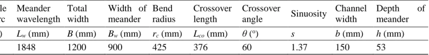
Water depth conditions for simulations were one in-bank case and two overbank cases, namely 7

Dr = 0.15 and Dr = 0.50, where Dr is the relative depth defined in Table 2. These were chosen

8

because the secondary flow structure in the main channel, and the shearing mechanisms 9

between the main channel flow and the flood plain flow, were of particular interest. 10

Measurements were conducted at section numbers 1, 3, 5, 7, 9, 11 and 13 (Fig. 1). The 11

hydraulic conditions of the selected cases are specified in Table 2. 12

Table 2. Hydraulic conditions of the experiments of Muto (1997) selected for the LES. 13 Depth condition Discharge Water Depth Relative depth Relative depth Mean velocity Friction velocitya Reynolds numberb Froude numberc Dr Q (·10-3_m3_s-1_{) H (m) H/h} Dr=(H-h)/H Us (ms -1₎ *

u

a.

u

5

3

Numerical Method and Computational Setup

The simulations were performed with the in-house code LESOCC2 (Large Eddy Simulation On 2

Curvilinear Coordinates). It is a successor of the code LESOCC developed by Breuer and Rodi 3

(1996) and it is described by Hinterberger (2004). The code solves the Navier-Stokes equations 4

on body-fitted, curvilinear grids using a cell-centred finite volume method with collocated 5

storage arrangement for the Cartesian velocity components. Second-order central differences are 6

employed for the convection as well as for the diffusive terms. The time integration is 7

performed with a predictor-corrector scheme, where the explicit predictor step for the 8

momentum equations is a low-storage three-stage Runge-Kutta method. The corrector step 9

covers the implicit solution of the Poisson equation for the pressure correction (SIMPLE). The 10

Rhie and Chow momentum interpolation (Rhie and Chow, 1983) is applied to avoid pressure-11

velocity decoupling. The Poisson equation for the pressure increment is solved iteratively by 12

means of the “strongly implicit procedure” of Stone (Stone, 1968). Parallelization is 13

implemented via domain decomposition, and explicit message passing is used with two halo 14

cells along the inter-domain boundaries for intermediate storage. 15

The subgrid-scale (SGS) stresses, resulting from the unresolved motions, are modelled using the 16

Smagorinsky subgrid-scale model (Smagorinsky, 1963) with a model constant Cs of 0.1. Such 17

an approach has been used successfully for similar flows by Hinterberger et al. (2007) and 18

Moncho-Esteve et al. (2017). For flows without homogeneous directions, as the present one, the 19

Smagorinsky model is more robust than other models like the dynamic Smagorinsky which 20

require some kind of smoothing of the model parameter (like time relaxation). Near the walls 21

Van-Driest damping is employed. 22

For the numerical calculation a global coordinate system was used (X, Y, Z), while for the data 23

analysis the quantities were transformed on a body-fitted coordinate system. According to the 24

definition in Shiono and Muto (1998), the x-axis is hereby along the centreline of the channel 25

bed, the y-axis along the span-wise and the z-axis along the vertical direction. The 26

computational grids consisted of ~ 5.8·106 _{grid points for the Bankfull case, ~ 7.2·10}6 _{for the Dr} 27

= 0.15 case and ~ 12.1·106 _{for the Dr = 0.50 case. More details of the grids are specified in} 28

Table 3. 29

30

Table 3. Computational grids for the simulated cases. 31

Case Used Mesh:

Grid Points in x-, y-, z-

Total Grid Points Bankfull 1200·110·44 5,808,000 Dr = 0.15 960·90·40 = 3,456,000 (in-bank) 960·390·10 = 3,744,000 (flood plain) 7,200,000 Dr = 0.50 960·90·40 = 3,456,000 (in-bank) 960·390·23 = 8,611,200 (flood plain) 12,067,200 32

6 1

Fig. 2. Detail of the grids in a cross section of the compound meander used in the LES 2

simulations. (a) bankfull case, (b) Dr = 0.15 case and (c) Dr = 0.50 case. (1.5-colum fitting 3

image)

4 5

The computational grids are uniform along the centreline in x-direction and stretched in y- and 6

z-directions to achieve a better resolution of the near wall motions. The grid sizes in terms of

7

wall units near the walls (∆y+ =∆z+) and the maximum value of

∆x

direction are shown in Table 4 for each one of the computational cases. The stretching ratio is 9

kept to a fix value of 1.03 in all cases. A view of the grid cross section for each of the cases is 10

shown in Fig. 2. Only one wavelength of meander was computed and periodic boundary 11

conditions were defined in the entrance and exit of the meander. A no-slip condition, with 12

smooth surface, was implemented at the bottom boundary and lateral walls jointly with the 13

Werner-Wengle wall model.In this way, with the wall function of Werner and Wengle (1993) 14

the shear friction at the first cell near the wall is calculated using the 1/7th_{-power law of the} 15

instantaneous velocities. Moreover, a rigid-lid assumption was used for the free surface, which 16

means that a symmetry condition is introduced, whereby the velocity normal to the surface and 17

the velocity gradient parallel to the surface are set to zero; hence, the surface is approximated by 18

a free-slip rigid surface. This method has been successfully employed in previous studies of 19

similar configurations (Stoesser et al., 2008; Brevis et al., 2014 and Moncho-Esteve et al., 2017). 20

The employed grid resolution is reasonable for a non-wall-resolving simulation. This is 21

supported by the good agreement with experimental data that will be shown in the following 22

7

sections. For comparison, Xu et al. (2013) employed a similar grid resolution in their 1

meandering open channel bend calculations while Brevis et al. (2014) employed a somewhat 2

finer grid resolution for a similar flow configuration. In addition, the grid resolutions employed 3

here are somewhat finer than those employed in a previous study by some of the present authors 4

(Moncho-Esteve et al., 2017). In the latter case the agreement with experimental data was also 5

good. Therefore, we are confident that the grid resolution employed here is good enough to 6

study the mean flow and turbulence characteristics of the flow under consideration. 7

Table 4. Grid sizes in terms of wall units near the wall (∆y+and ∆z+) and maximum grid sizes 8 in stream-wise direction (∆z+). 9 Case ∆x+ ∆y+ _∆z+ Bankfull 29 12 12 Dr = 0.15 in-bank 32 9 9 flood plain 30 12 12 Dr = 0.5 in-bank 52 15 15 flood plain 44 16 16

4

Results & Discussion

10

4.1

Streamwise Flow

11

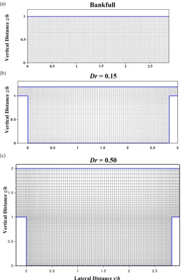
All the velocities in this section are normalized by the average velocity Us = Q/A, Q being the

12

flow rate and A being the transverse section of the flume. The Figure 3 presents a qualitative 13

comparison of the mean streamwise velocity

u

cases, where angular brackets denote average over time. For the sake of brevity, only 15

Section No. 09 is shown for comparison with the experimental data. In general a good 16

agreement was found between simulations and experiments at the meandering cross-sections. In 17

this figure the results of the simulations are shown on the left and the experimental results on 18

the right. 19

In the Bankfull case (Fig. 3, top panels) the highest velocities, with a magnitude over 1.3Us, are

20

found near the inner bank (convex channel wall) in the bend apex (not shown). As the flow 21

advances towards the second half of the curve, the core of the maximum velocity moves 22

towards the outer bank (concave channel wall), and the distribution of the velocity are softened. 23

In the middle of the crossover region of the meander a flow region superior to 1.2Us reaches the

24

outer wall (not shown). After the flow enters the second curve (Section No. 09) the maximum 25

velocity is still moving towards the right sidewall. This tendency matches the experimental data 26

accurately. Coinciding with the previous studies (Chang, 1971; Moncho-Esteve et al., 2017) the 27

maximum value of the streamwise velocity seems to be placed in the entrance of the curve, near 28

the Section No. 09, where values over 1.3Us are reached. Overall, a correct consistency in both

29

shape and intensity on the contours of the mean streamwise flow is appreciated, although the 30

simulation underestimates slightly the values compared to the experimental results. 31

For the Dr = 0.15 case (Fig. 3, middle panels) regions of high velocity are formed near both 32

walls in the apex of the curve (not shown), while the central part is occupied by a lower velocity 33

area. Throughout the meander, large regions can be found in which the velocity is higher than 34

Us. This suggests that the flow in the meander with a low flood water depth still maintains a

35

dominant longitudinal component (Shiono and Muto, 1998). At the bend apex (not shown), 36

areas of slower flow motion can be seen near the bed in the middle section, which are clearly 37

8

influenced by the secondary flow structures through the meander (see Fig. 10 and corresponding 1

discussion). Moreover, in the crossover region (Section No. 05-09), a steep velocity gradient 2

related to the flow entering from the upstream flood plain is developed in the vertical direction 3

near the bankfull level. This area develops laterally as it proceeds in the crossover region. The 4

mean flow patterns described are observed in both the contours from the simulations and from 5

the experiments. The agreement between the two is good, although there is a small 6

overprediction of the maximum velocities in the simulation. Comparing the contours in Bankfull 7

and Dr = 0.15 cases (Figs. 3, top and middle panels), it can be observed that even a low flood 8

water depth influences significantly the flow patterns within the meander. This is particularly 9

clear in the crossover region. 10

11

Fig. 3. Mean streamwise velocity

u

12

and Dr = 0.50 (bottom panels). Left: LES simulation; Right: experimental measurements by 13

Muto (1997). (2-colum fitting image) 14

15

Regarding the case Dr = 0.50 (Fig. 3, bottom panels), in the crossover region of the meander, 16

and on top of it, a velocity gradient can also be observed, due to the inflow from the floodplain 17

into the meander. It can be seen an area of considerable low velocity in the right-hand wall of 18

the outlet of the curves (Sections No. 03 and No. 5 (not shown)). Moreover, the in-bank flow 19

has a streamwise velocity value throughout the meander channel under Us, which suggests that,

20

with high levels of flooding, a dominance of the floodplain flow over the meander ensues 21

(Shiono and Muto, 1998). There is a good correlation between the simulation and the 22

experimental features described above. Similar to the Dr = 0.15 case, the velocity value in the 23

9

simulation seems to be slightly overestimated. Comparing Dr = 0.15 and Dr = 0.50 cases (Figs. 1

3, middle and bottom panels), it is noteworthy that the flow patterns within the meander (z/h<1) 2

are rather similar, however, the velocity levels are different. While with the low water depth 3

(Fig. 3, middle panels) the velocities within the meander may be higher than Us, with the high

4

water depth (Fig. 3, bottom panels) the velocities are significantly lower. As Shiono et al. (2008, 5

2009a, 2009b) demonstrated, sediment transport rate decreases from in-bank flow to Dr = 0.3 6

which means that in the meandering channel the velocity decreases as well. 7

Some deviations between the experimental data and the simulation results are found near the 8

free surface. This might be due to the use of the rigid-lid assumption for the free surface. 9

Besides, in the simulation some wiggles can be observed in the sections where there is supposed 10

to be a strong flow interaction between the meander flow and the flood plain flow (Sections No. 11

05 and No. 09). This indicates that a somewhat finer resolution might have been required to 12

avoid these oscillations, especially in the region of the interface between meander and flood 13

plain. However, since the overall agreement with the experimental data is very good we can 14

infer that the impact of the wiggles is minor. Finally, recall from Fig. 1 that sections 1 and 13 15

(not shown) present mirror symmetry with respect to the midline of the cross section since these 16

sections are the opposite apices of the periodic meander. This mirror symmetry indicates that 17

the simulations have been run long enough for the statistics to converge. 18

4.2

Flood Flow Angle

19

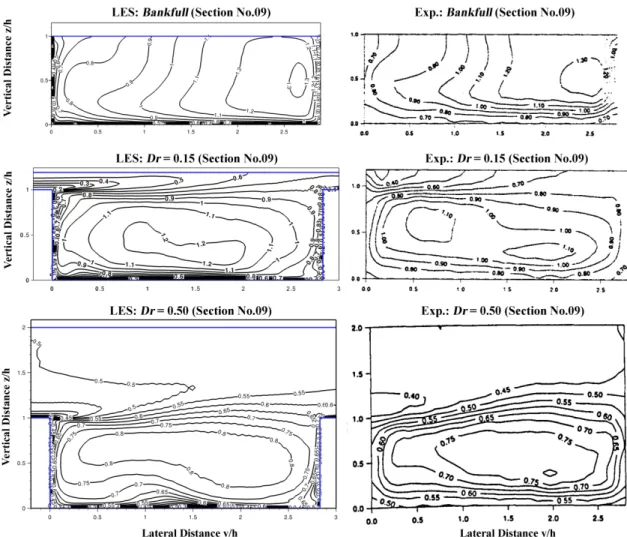
Fig. 3 have provided a qualitative comparison between experiments and simulations. A 20

quantitative comparison is provided in Fig. 4. This is done by resolving the floodplain flow into 21

two components as it was done by Shiono and Muto (1998), see their Fig. 7. The angle between 22

these two components, θ, can be obtained as θ = tan-1₍

_v

_u

_v

velocity and u the aforementioned mean streamwise velocity. Shiono and Muto (1998) 24

reported vertical profiles of the flow angle for the case Dr = 0.50 at two spanwise locations, y/h 25

= 0.56 (inner side of the meander channel) and y/h = 2.55 (outer side). Fig. 4 displays these 26

profiles at several sections, including both experimental data and simulation results. Shiono and 27

Muto (1998) stated that especially at y/h = 2.55, Sections No. 05 and 09, the mean flow angles 28

do not coincide with the meander channel angles (60o_{). The authors indicate that the main} 29

channel fluid runs into the flood plain. On the other hand, the mean flow angles at Sections No. 30

01, 03 and 05 are less than the channel angles (0 o_{, 30} o _{and 60} o _{respectively), which indicates} 31

that the floodplain flow is diverted into the main channel flow direction. However, the angles at 32

Sections No. 09 and 11 (60 o _{and 30} o_{) are greater than the channel angle, representing a flood} 33

plain flow diversion outwards towards the flood plain. These features related with the expansion 34

and contraction (i.e. a phenomenon showed by Kiely, 1990) of the flood plain flow entering and 35

escaping respectively from the main channel flow are shown and clarified in the next sections. 36

10 1

Fig. 4. Mean flood flow angle to meandering cannel with depth variation for Dr = 0.50, (a) y/h 2

= 0.56, (b) y/h = 2.55. (2-colum fitting image) 3

11

As it can be seen in Fig. 4, the predicted mean flow angle profiles show very good agreement 1

with the measurements. Although the trends of the profiles are to a large extent reproduced by 2

the model, significant differences were found in the in-bank flow of Section No. 05, specially in 3

the outer side of the meander (y/h = 2.55). In this section, the largest discrepancies with respect 4

to the measured flow angle are 19.15 deg. at z/h = 0.4. In the inner side of the meander channel 5

(y/h = 0.56), the mayor differences were found in the same section at z/h = 0.3. The deviation 6

may stem from the steep gradient that exists in this region, related with the aforementioned 7

entering and escaping flow as well as the complex secondary motions due the flood plain flow. 8

However, in general the good agreement with the flow angle supports the assumption that the 9

grid resolution is sufficient to capture major effects in the mean flow field. 10

4.3

Fluctuations and Turbulent Kinetic Energy

11

The root mean square of the streamwise and lateral velocity fluctuations, u' and v' 12

respectively, were obtained and compared with the experimental measurements (Muto, 1997). A 13

prime denotes velocity fluctuation. Statistics were collected during 500 dimensionless time units 14

H/Us. In the following velocity fluctuations are normalized with the friction velocity

* u . The 15

calculated u for each experimental case is listed in Table 2. The simulations were performed * 16

using a horizontal water surface and a horizontal channel bed. This is a general technique used 17

in CFD to model flow in channels. The driving force is a pressure gradient, instead of the 18

gravity. Thus, in the case of the simulations, the friction velocity was obtained as 19 2 / 1 . * 1 ) ( _      = R dx dp u _sim ρ (1) 20

where ρ is the density, p is pressure and R is the hydraulic radius. The values obtained for the 21

Bankfull, Dr = 0.15 and Dr = 0.50 simulations were 0.0166, 0.0116 and 0.0210 ms-1 22

respectively, which are reasonably consistent with the experimental ones (Table 2). 23

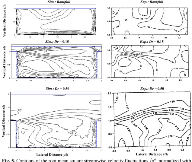
Figures 5 and 6 present a qualitative comparison of the velocity fluctuations for the Bankfull, 24

Dr = 0.15 and Dr = 0.50 cases. For the sake of brevity, only Section No. 09 is shown. For the

25

other sections a similar agreement was found between simulations and experiments. 26

In the Bankfull flow (Fig. 5, top panels), u' reaches values up to 3 u* along the inner bank of

27

the bends (not shown). Besides, another area of high u' appears near the channel bed and to a 28

lesser extent next to the outer banks. The later is not found in the experimental data, most 29

probably due to the resolution near the walls. Regarding the lateral component v' (Fig. 6, top 30

panels), large values appear at the channel centre near the water surface in the curves, where it 31

is about 2 u*. Generally, a correct consistency in both shape and intensity on the contours of the

32

streamwise and lateral velocity fluctuations is appreciated, although the simulation 33

underestimates slightly the experimental results. 34

12 1

Fig. 5. Contours of the root mean square streamwise velocity fluctuations u' normalized with 2

the u_* in Section No. 09 for the Bankfull (top), Dr = 0.15 (middle) and Dr = 0.50 (Bottom). 3

Left: LES simulation; Right: experimental measurements by Muto (1997). (2-colum fitting 4

image)

5 6

In the Dr = 0.15 case (Fig. 5 and 6, middle panels) the results show a good agreement with the 7

experimental results by Muto (1997) except near the water surface. The maximum values are 8

around 2.25 u* and they appear in shear layer regions where the flow interaction occurs by the

9

floodplain flow entering the main channel in the upper left corner of Sections No. 05-09. This 10

interaction is also well reproduced by the LES results. This area is developed over the channel 11

width, increasing in size. In addition, both the shape and magnitudes of u and ' v' correspond 12

well with each other in most of the cross-section. 13

13 1

Fig. 6. Contours of the root mean square lateral velocity fluctuations v' normalized with the 2

*

u in Section No. 09 for the Bankfull (top), Dr = 0.15 (middle) and Dr = 0.50 (Bottom). Left: 3

LES simulation; Right: experimental measurements by Muto (1997). (2-colum fitting image) 4

5

In the case of Dr = 0.50 (Fig. 5 and 6, bottom panels), the upper layer flow seems to influence 6

significantly the turbulent flow structure. For this water depth condition, the lower layer is more 7

turbulent than the upper layer, which is clearly seen in the crossover region. The area of large 8

turbulent intensities expands slightly into the upper layer, with values over 2.5 u*. For both

9

velocity components, this area of high turbulent intensity is found roughly at the same central 10

location. Although the velocity fluctuations seem to be slightly overestimated in the 11

simulations, the patterns described above are qualitatively similar in both the experimental data 12

and the simulations results. Like for the mean streamwise velocity components (Fig. 3, bottom 13

panels), some small wiggles can be observed in the sections where there is a strong flow 14

interaction between the meander flow and the flood plain flow (Sections No. 05 and No. 09). 15

As Muto (1997) noticed, the turbulent shear layer generated at the bankfull level is most 16

dominant for the bankfull flow (Dr = 0.15 and Dr = 0.50 cases), leading to a high turbulence 17

intensity, both in streamwise direction and laterally and, accordingly, both 'u and v' reflect 18

such a feature. 19

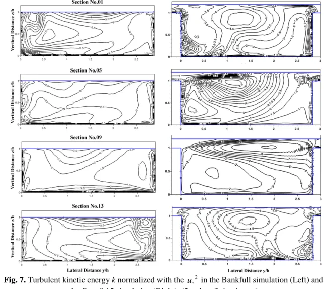
Moreover, in this section, a qualitative comparison of the turbulent kinetic energy k is provided 20

in Fig. 7 and 8 between the cases Bankfull, Dr = 0.15 and Dr = 0.50. Only Sections No. 01, 05, 21

09 and 13 are shown for comparison. The turbulent kinetic energy is given by 22

14

(

)

Since in the experiments the vertical component was not measured in the whole area of the cross 2

sections (Muto, 1997), only the data from the simulations is presented. In the following k is 3

normalized with the square of the friction velocity u . _*2

4

In the Bankfull case (Fig. 7, left panels), the highest values of k are found near the side walls 5

and the bed of the channel, due to the strong shear found in these regions. Also the level of 6

turbulence is higher near the free surface than in the core of the channel. Although it is difficult 7

to observe in the figure, the maximum value of k reaches values about 6.9 u*2. As mentioned

8

before, Sections No. 01 and 13 should present mirror-symmetry with respect to the midline and 9

indeed the patterns obtained from the simulations are almost symmetric. 10

11

Fig. 7. Turbulent kinetic energy k normalized with the 2 *

u in the Bankfull simulation (Left) and

12

the Dr = 0.15 simulation (Right). (2-colum fitting image) 13

14

In the case Dr = 0.15 (Fig. 7, right panels) the area where the higher turbulence values are 15

gathered is located in the upper part of the meander through its straight section, corresponding 16

to the interaction between the inner and the outer flows. This is particularly clear in Section No. 17

09, where a region of hight turbulence level is found near the meander top (z/h ~ 1). Values 18

higher than 9.0 u*2 are reached. It is possible to notice that in the bed, near the outer banks of the

15

curves (right lateral wall at Sections No. 01 and 05 and left lateral wall at Sections No. 09 and 1

13), areas with k lower than 1.5 u*2 appear. Just as Muto (1997) noted, due to the secondary

2

flow being very weak in this area (as will be shown below), deposit of sediments in natural beds 3

can occur. 4

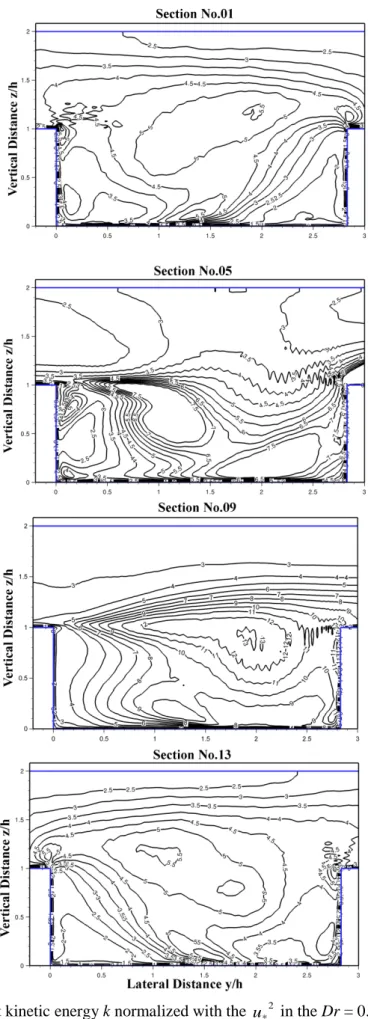
For Dr = 0.50 (Fig. 8), a similar behaviour to the Dr = 0.15 case is observed, keeping the core of 5

maximum k slightly under the level of the floodplain bank and taking more space. The 6

maximum values surpass in this case 13 u*2. Throughout the crossover region (see Section No.

7

05), high values of k can be seen in the flood plain flow, near the outline of the curve (y/h = 3, 8

z/h ~ 1).

9

Regarding the distribution of k, one of the key differences between the Dr = 0.15 and Dr = 0.50 10

cases is the position of the core of the turbulent area. In the shallow overbank flow, such area 11

remains close to the water surface, but nevertheless in the deep flooding case it is located mostly 12

below the bankfull level, 0.5<z/h<1.0. The study of Muto (1997) did not clarify whether the 13

former's characteristic was related to the depth conditions or whether it could be due to the 14

fairly shallow flooding depth which was not enough to give a proper measurement resolution in 15

the vertical direction. The fact that this feature was well drawn by the numerical results leads us 16

to state a clear correlation with the water depth and this turbulent core. 17

16 1

Fig. 8. Turbulent kinetic energy k normalized with the u in the Dr = 0.50 simulation. (2-_*2

2

colum fitting image)

17 1

Fig. 9. Turbulent kinetic energy k normalized with the u in a horizontal plane (z/h = 0.9) of _*2

2

the meandering channel. Top: Dr = 0.50 case, middle: Dr = 0.15 and bottom: Bankfull. (Colour 3

should be used in print) (2-colum fitting image)

4 5

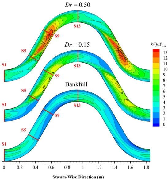
Figures 7 and 8 show that the floodplain flow changes the structure of the turbulent kinetic 6

energy patterns near the interface with respect to the bankfull case. Therefore, it is interesting to 7

study the longitudinal patterns near this interface. Figure 9 shows the contours of the normalized 8

turbulent kinetic energy in a horizontal plane (z/h = 0.9) of the main channel for the Bankfull, 9

Dr = 0.15 and Dr = 0.50 cases. The corresponding sections shown in the previous Figs. 7 and 8

10

are specified here for better interpretation. In the case of Bankfull, the maximum values of k 11

appear near the bend apices of the meander. As mentioned by Muto (1997), these values are 12

related to the wall generated turbulence and the secondary flow generated turbulence, both of 13

which contribute mainly to the production of

u

'

v

'

flooding, the region with the highest k appears in the crossover region. This effect has a higher 15

intensity for Dr = 0.50 than for Dr = 0.15. In this area a very intense shear layer between the 16

flow in the flooding level and the flow throughout the meander is produced. This shear layer 17

generates additional turbulence due to the interaction and the mixing process between the 18

flooding flow and the meandering flow. In the case Dr = 0.15 a great influence in the wall 19

generated turbulence and the secondary flow in the meander must still exist, considering, as 20

18

Muto (1997) indicated, the k is related in the crossover region with the distribution of

u

'

'

v

contribution to the production of turbulent energy appears near the shear layer, which is more 3

correlated with the

v

'

meandering flow. 5

The aforementioned flow intrusion and the resultant interaction between the upper and lower 6

flows strongly affect the flow structure in compound meandering channels during floods (Muto, 7

1997). Specifically, this relates to the internal shear at the bankfull level for overbank flows, 8

which in turn is the dominant mechanism for turbulence generation in these cases. Moreover, 9

this feature induces the horizontal layer of turbulence nature in the crossover region, which is 10

the main factor for production of secondary flows. The results showed here (Fig. 9) cover the 11

shape and form of such turbulent shear layer for the two water depths. 12

4.4

Secondary Flow

13

The mean secondary current vectors of Sections No. 01, 03, 05, 07, 09, 11 and 13 are presented 14

in Figs. 10 and 11 for the Bankfull, Dr = 0.15 and Dr = 0.50 cases. 15

For the in-bank flow case (Fig. 10, left panels), a big clockwise circulation cell can be observed 16

near the inner bank (left lateral wall) at Section No. 01. This secondary current comes from the 17

previous bend and it is similar in form and magnitude as the one shown at Section No. 13. 18

While the flow near the bed moves from the outer to the inner-bank (right to left), the flow close 19

to the surface moves in the opposite direction. In addition to the centre-region cell a small cell 20

near the outer-bank (right lateral wall) is present, rotating in an anti-clockwise direction. The 21

flow at the bottom of the channel has already switched sign at Section No. 11. In this position, 22

the small outer-bank cell rotating in anti-clockwise direction mentioned above becomes the 23

centre-region cell. Close to the surface of the inner bank, rotating in a clockwise direction, the 24

previous centre-region cell can be seen decreasing in strength. This behaviour seems to confirm 25

that these secondary currents are a process of the growth and decay of two cells of the primary 26

vortex, which has been also shown and discussed in Moncho-Esteve et al. (2017), for a similar 27

flow configuration. The agreement (comparison not shown) with the experimental results (Muto, 28

1997) is remarkably good. 29

19 1

Fig. 10. Mean secondary flow vectors in the Bankfull simulation (Left) and Dr = 0.15 2

simulation (Right). (2-colum fitting image) 3

20

The effect of the floodplain flow completely changes the mechanisms of the secondary currents 1

within the meander. For the Dr = 0.15 case (Fig. 10, right panels), a big shear-generated anti-2

clockwise recirculation cell could be observed at Section No. 01 in the vicinity of the inner bank 3

which comes from the previous bend; this recirculation is weakened by the centrifugal effects 4

throughout the bend. In this case, a small counter clockwise cell is also noticeable at the outer 5

bank and near the channel bed. However, both circulations disappear suddenly along the next 6

reach by entering floodplain flow that changes completely the secondary circulation patterns 7

inside the meander. In order to evaluate where this transition takes place additional cross-8

sections were studied (results not shown). These sections represent the point where the 9

aforementioned big shear-generated recirculation cell, which was generated in the previous bend, 10

disappears completely. Fig. 12a shows the additional cross-sections between which the 11

transition occurs for the case Dr = 0.15. Thus, the change occurs at an angle of roughly 24º from 12

the bend apex. At this moment, the meander flow takes an oblique direction to the main 13

floodplain stream, which produces a high velocity above the bankfull level in the crossover 14

region and a vigorous expansion-contraction phenomenon occurs when the floodplain flow 15

enters into the meander section and vice versa. From that section on (namely Section No. 02.9), 16

a big clockwise centre-region cell appears (from Section No. 05 to 09 in Fig. 10, right panels). 17

This big secondary current progresses downstream towards the inner wall of the next bend 18

(Section No. 09). In the latter part of the meander, as the meander takes a parallel direction to 19

the floodplain mainstream, the floodplain flow entering the meandering channel decreases and a 20

counter rotation cell appears, similar to Section No. 01. The progress of the primary vortex 21

generated by the floodplain flow along the meandering channel is very well predicted by the 22

LES simulation (comparison with the experiments of Muto not shown). The fact that the 23

secondary circulations within the meandering channel change completely as soon as there is 24

some floodplain flow can be understood by simple analogy with the flow in a lid driven cavity 25

(Koseff and Street, 1984). While the flow along the meander has the same direction as the 26

floodplain flow, the secondary patterns are little affected. As soon as the orientation of the 27

meander changes sufficiently, the floodplain flow acts as a driving mechanism for the secondary 28

currents, imposing their rotation. 29

21 1

Fig. 11. Mean secondary flow vectors in the Dr = 0.50 simulation. (2-colum fitting image) 2

3

For the Dr = 0.50 case (Fig. 11), the flow behaves in a simpler way because the influence of the 4

cross-over flow of the floodplain mainstream is more pronounced. At Section No. 01, almost no 5

recirculation cell is noticeable. However, at an angle of 16º (see Fig. 12b), a big centre-cell 6

recirculation begins to be formed by the entrance of floodplain flow. Thus, almost the whole 7

cross-sectional area is occupied by only one dominant secondary flow cell which displaces its 8

centre towards the inner bank at Sections No. 07 and 09. From that section on, the secondary 9

flow decays and it has almost vanished at Section No. 13. The expansion and contraction 10

processes are also visible around Section No. 05. The situation is similar although not so 11

marked as regards to the Dr = 0.15 case. The progress of the primary vortex generated by the 12

22

floodplain flow along the meandering channel is once again very well predicted by the LES 1

simulation (experimental data of Muto not shown). 2

3

Fig. 12. 2D-streamtraces in additional cross-sections where entering floodplain flow cancelled 4

completely the previous shear-generated vortex inside the meander. (a) Dr = 0.15 case, (b) Dr = 5

0.50 case. (2-colum fitting image) 6

7

In Fig. 13 and 14, different views of the three-dimensional streamlines of the mean flow are 8

shown for the Dr = 0.15 and 0.50 cases. The streamlines are coloured with the normalized 9

turbulent kinetic energy. This figures illustrate the phenomenon of the interaction and mixing 10

process between the floodplain mainstream and the in-bank meandering flow, whose 11

consequences are mainly the horizontal shearing and the downstream effects of crossover flow. 12

These pictures confirms the tendency (Shiono and Muto, 1998) of the flow within the main 13

channel below the bankfull level to follow the meander channel, while above the bankfull level 14

it tends to follow the valley direction. As it can be seen, the flow enters the meander (expansion 15

behaviour) in the inner margin of the bends and begins to swirl according to the secondary 16

currents previously explained. It is also noticeable how the contraction (escaping flow) 17

phenomenon occurs near the outer bank of the bends when the flow from the main channel 18

reaches the floodplain again before the interaction with the meander flow. The latter two 19

features are in agreement with the description of Sellin et al. (1993), who showed velocity 20

vectors in the main channel and the flood plain along a compound meander channel and pointed 21

out the dropping and recirculation of the upper flow in the main channel. In the case of the Dr = 22

0.15, it can be seen how the main floodplain flow seems to be more conditioned (significant 23

deflection is shown) by the in-bank secondary flow through the straight section, whereas in Dr 24

= 0.50 case it appears to flow smoothly over the main channel, which means that with a deep 25

condition the interaction is less important and the two layers are less dependent on each other. 26

In both cases and according to the Figs. 7 (right panels) and 8, higher values of the turbulent 27

kinetic energy can be seen in the middle of the crossover region of the meander and the entrance 28

of the curves (Section No. 09). Moreover, the contribution of the turbulent kinetic energy seems 29

to concentrate within the main meandering channel for Dr = 0.15 more than in the floodplain. 30

On the other hand, greater turbulence values are gathered not only under the level of the 31

floodplain bank and taking more space but also throughout the flood plain for Dr =0.50. 32

23 1

Fig. 13. Different views of the 3D stream traces of the mean flow coloured with the normalized 2

turbulent kinetic energy k/ 2 . *)

(u _sim for Dr = 0.15 case. (Colour should be used in print) (1.5-3

colum fitting image)

4 5

24 1

2

Fig. 14. Different views of the 3D stream traces of the mean flow coloured with the normalized 3

turbulent kinetic energy k/ 2 . *)

(u _sim for Dr = 0.50 case. (Colour should be used in print) (1.5-4

colum fitting image)

5 6

A detailed analysis of this process is illustrated in Fig. 15. The figure shows some plots of the 7

mean flow vectors and the normalized turbulent kinetic energy k/ 2 . *)

(u _sim near the outer side of 8

the meander channel and the flood plain edge roughly in Section N. 05, for Dr = 0.15 and Dr = 9

0.50 cases. A small recirculation pattern appears around Section No. 05 (Fig. 15, middle panels) 10

at the floodplain edge region. The pattern seems to be bigger for Dr = 0.50 (Fig. 15b) compared 11

with the Dr = 0.15 case (Fig. 15a). This indicates that when the flood water depth increases, this 12

25

interaction between the flooding and the main channel meandering flow increases. An area 1

producing high turbulent energy is easily recognized in the vicinity of the recirculation (Fig. 15, 2

top panels), over the flood plain bank and near the concave side of the meander wall. This 3

energy reach values up to 13 u*2 for the Dr = 0.15 and exceeds 29 u*2 in the Dr = 0.50 case. A

4

similar turbulent area was noticed by Muto (1997) by means of the depth averaged turbulent 5

kinetic energy on the flood plain next to the bend exit. Muto also summarized the findings of 6

Imamoto and Fujii (1975), who stated that turbulence becomes more intense when the flow 7

passes over a forward step, being this tendency more noticeable near the bed; our results agree 8

with their results and support the evidence that this highly turbulent fluid comes from the main 9

channel. Moreover, the mean flow vectors at the flood plain edge (Fig. 15, bottom panels) 10

follow the path towards the edge of the outer bank of the meander channel. This trend occurs in 11

both cases (Dr = 0.15 and Dr = 0.50) in a narrow area alongside the floodplain edge region. 12

This area corresponds to the aforementioned recirculation and ranges from the second half of 13

the bend (between Section No. 03 and No. 05) to the first part of the crossover region (between 14

Section No. 05 and No. 07). This area agrees with the vigorous expulsion of the inner channel 15

water (contraction process) described by Ervine et al. (1994) and Wormleaton et al. (2004), 16

which induces the recirculation (Fig. 15, middle panels) and the consequent tendency of vectors 17

to move towards the edge of the outer bank. This highly turbulent mechanism, not seen before, 18

could be related to the erosion mechanisms (producing strong scour in this zone) and the 19

channel migration present in this kind of flow. Although the intensity of the vectors appears to 20

be qualitatively similar in both cases (Fig. 15, bottom panels), recirculation and turbulence are 21

greater for Dr = 0.50 (Fig. 15d). In this sense, for higher levels of flooding, a bigger influence of 22

this mechanism in the scouring process is expected. 23

26 1

Fig. 15. Detail of the outer side of the meander channel near Section N. 05. Top: normalized 2

turbulent kinetic energy k/ 2 . *)

(u _sim . Middle: close up view of the mean secondary flow vectors. 3

Bottom: top view of the mean flow vectors in the first cells next to the floodplain bed. (a, c) Dr 4

= 0.15 case, (b, d) Dr = 0.50 case. (2-colum fitting image) 5

6

Although there are clear significant differences in the flow configuration, the aforementioned 7

phenomenon of flow expansion (flow entering from the flood plain into the meander channel) 8

could be related to a separation of flow such as those produced by dune formation (Shiono et al., 9

2008; Stoesser et al., 2008). In this process, the flow over the dune crest creates a large 10

separation zone, with which is associated a turbulent free shear layer generating large scale 11

eddies that travel through the flow domain. In our cases, this behaviour appears to weaken when 12

the flood increases (Dr = 0.50). In the Dr = 0.50 case, the mean flow is more likely to just travel 13

over the meandering flow, generating an in-bank flow structure with a primary gyre which is 14

more similar to the one observed in the flow around an emerged dead zone sequence (Brevis et 15

al., 2014; Weitbrecht, 2004). However, at a depth near Dr = 0.50, Shiono et al. (2008) showed 16

dunes which were caused by a number of secondary flows in sequence along the meandering 17

channel. On the other hand, the phenomenon of contraction (escaping flow from the meander 18

27

onto the flood plain) near the cross-over region could be connected to the flow behaviour over 1

the cylinder top. Hain et al. (2008) and Palau-Salvador et al. (2010) studied in depth the flow 2

around finite-height cylinders and showed that the flow separates at the leading edge, yielding a 3

recirculation. In fact, the flow picture over the cylinder top sketched by the last mentioned 4

authors (Fig. 16 in Palau-Salvador et al., 2010) is quite similar as the one showed in this study 5

(Fig. 16). 6

4.5

Bed Shear Stress

7

In natural rivers, the bed shear stress is important in determining the bed erosion and the 8

sediment transport (Shan et al., 2016). The bed shear stress is hardly ever measured in 9

experiments because of the inherent measurement difficulty; however, it is easier to obtain from 10

the computational data. This section therefore presents the bed shear stress at the bottom walls 11

as an application of the initial step in the erosion processes. To do this, we estimate this 12

parameter in the first cells of the mesh next to the bed in the meander and floodplain making use 13 of the equation 14 dn du_t w µ τ = (3) 15

where, µ is the dynamic viscosity,

u

n the distance from the bed. The bed shear-stress is normalized with the total bed shear stress

17

obtained from the resulting pressure gradient 18 dx dp R t = τ (4) 19

where R is the hydraulic radius. As a cautionary note, recall that the present simulations are not 20

wall-resolving. This means that the bed shear stress values discussed below can be only 21

considered as an estimation of the real values. We believe, however, that the trends and 22

differences observed between the three cases are reliable, and would differ little if obtained with 23

wall resolving simulations. 24

Fig. 16 shows the distribution of the normalized bed shear stress of the Bankfull case. Note that 25

for brevity the shear stress is not shown in the meandering lateral walls, although its value is not 26

negligible. The maximum value of the bed shear stress occurs in the curves, close to the inner 27

bank, reaching values of up to 0.9

τ

shifted and smoothed towards the outer edge of the curves. In the straight sections a small area 29

of maximum shear appears at the right margins, just outside the curves. 30

Fig. 17 shows the distribution of the normalized bed shear stress in the Dr = 0.15 case, both in 31

the meander and in the floodplain. Within the meander, an effect similar to the Bankfull case 32

occurs, reaching values up to 0.9

τ

τ

the left margins of the straight sections, and in the central areas of the curves near the inner 34

banks, coinciding with low velocity zones in the bed. Likewise, in the floodplain the greatest 35

bed shear stresses of the domain occur, reaching values up to 1.1

τ

concentrated in the zones where there is a greater interaction between the meander flow and the 37

floodplain flow, which has its origin in the strong acceleration due to the contraction and 38

expansion of the flow. As was pointed out by Wormleaton et al. (2004), the great expulsion of 39

28

the flow in this case induces local high velocities near the main channel outer bank, which are 1

related to the risk erosion in that area. 2

Finally, in the Dr = 0.50 case (Fig. 18), the maximum bed shear stresses of the entire domain 3

are produced within the meander, reaching values higher than 1.1

τ

occur, unlike in previous cases, in the straight sections of the meander, occupying much of the 5

bed due to the big center-cell originated by the flow coming from the floodplain. At the exit of 6

the curves of the meander, large areas of low shear (almost 0.0

τ

due to the low velocities in these sections. Within the floodplain, the bed shear stresses appear 8

to be concentrated below the meander margins that lie downstream of the flow direction of the 9

flooded plane, although their contribution is much lower than in the shallow case. The effects of 10

bed shear stress seem to be more intense within the meander as the level of flooding increases. 11

In this case and, as we mentioned earlier, the influence of the expulsion of water on to 12

floodplain is less than in the Dr = 0.15 case. On the other hand, as was illustrated by 13

Wormleaton and Ewunetu (2006), in deep floodplain, a strong shear-driven recirculation 14

through the meandering crossover region can cause deep scour in this area. 15

16

17

Fig. 16. Normalized bed shear stress τ (

τ

τ

should be used in print) (1.5-colum fitting image)

19 20

29 1

Fig. 17. Normalized bed shear stress (

τ

τ

should be used in print) (1.5-colum fitting image)

3 4

5

Fig. 18. Normalized bed shear stress (

τ

τ

should be used in print) (1.5-colum fitting image)

7 8

In order to provide a more quantitative comparison between the cases, Figure 19 shows profiles 9

of the normalized bed shear stress distributions at the crossover region and the first half of the 10

second bend (i.e Sections No. 03, 05, 07 and 09) for all three simulated cases. In the case of the 11

Bankfull flow, coinciding with the maximum value of the streamwise velocity (Fig. 3, top 12

panels), the maximum value of 0.87

τ

No. 09) near the inner wall. Except in Section No. 03, higher values are kept near the right bank 14

all over the meander. Regarding the Dr = 0.15 case, the maximum value of 2.42

τ

the end of the first bend (Section No. 05) near the right bank, at the floodplain edge region. 16

Similar feature (2.27

τ

30

water ejection (contraction process) towards the flood plain in the outer part of the curve. 1

Moreover, it might be related to the recirculation described above (Fig. 15) and therefore to the 2

erosion mechanisms and channel migration. In the other sections of this shallow flooding case, 3

higher values are always located near the right bank, at the floodplain edge region. The latter 4

coincides with the the flood plain flow crossing over the main channel flow in the crossover 5

region when it surpasses the right bank. Similar to the Bankfull case, in the main channel area, 6

higher values are kept near the right bank throughout the meander (except in Section No. 03). 7

Finally, for the Dr = 0.50 the maximum value of 1.49

τ

(Section No. 07) near the right bank, at the floodplain edge region. The last phenomenon 9

coincides with the the flood plain flow crossing over the main channel flow in the crossover 10

region when it surpasses the right bank. Although the higher values are located in this case in a 11

thin layer of the floodplain edge region, similar high values are also found in the main channel 12

bed, although its extension is greater. Along the same main channel bed, its shear profile 13

describes a shape very diffent from the Bankfull and Dr = 0.15 cases. In the deeper flow case 14

there is a sinusoidal profile, which maximum values seems to be related to the center of the 15

primary vortex (Fig. 11) throughout the meander. This relates to the aforementioned deep scour 16

area (Wormleaton and Ewunetu, 2006), caused by such strong shear-driven vortex in the 17

crossover region. 18

31

Fig. 19. Normalized bed shear stress (

τ

τ

(b) Section No. 07, (c) Section No. 09, (d) Section No. 011. (Colour should be used in print) 2

(1.5-colum fitting image) 3

4.6

Implications in Natural Banks

4

The results presented in this paper have been obtained for a flow configuration which can be 5

considered as artificial. The present meander cross-section is rectangular and the ratio of width 6

to bankfull depth is about three. On the contrary, banks usually found in nature have irregular 7

cross-sections and are somewhat wider than the one studied here. In this context, it is worth 8

considering how representative the investigated configuration is for natural compound 9

meandering rivers. 10

First, secondary flow structures in the present configuration have an opposite sense of rotation 11

of the primary vortex at bend apices before and after inundation. This is consistent with the 12

secondary flows observed by Spooner (2001) who conducted experiments on a meandering 13

compound channel with natural bed forms, including mobile bed cases. A similar secondary 14

flow structure was reported by Wormleaton et al. (2004) who studied experimentally the flow in 15

a realistic main channel plan-form and dimensions, foodplain conditions and mobile bed. The 16

configuration may be considered as broadly representative of conditions that occur in natural 17

rivers. In the case of smooth floodplain, the flood plain flow created a strong vortex in the 18

crossover region which basically cancelled out the centrifugal circulation around the following 19

apex. 20

Concerning the horizontal turbulent shear layer, it has been shown that it is induced by the flood 21

plain flow crossing over the main channel flow in the crossover region. The presence and 22

relevance of such a shear layer have been also discussed in the literature for natural banks. For 23

example, in the study of Wormleaton et al. (2004) mentioned above, this was identified as one 24

of the main governing mechanisms for overbank flows. Moreover, Mera et al. (2014) and Mera 25

et al. (2015) performed experiments on a 1:20 physical Froude model of a real reach in River 26

Mero (Spain), for two depth conditions (Dr = 0.26 and Dr = 0.38). These authors also identified 27

the generation of a shear layer at the horizontal interface. 28

The interaction between floodplain flow and meandering flow was also reported by Mera et al. 29

(2015). In their study, they showed that the flow below the bankfull level visibly followed the 30

direction of the main channel, whereas the flood plain flow tended to follow the floodplain 31

direction bank. A realigment of the water circulation throughout the meander was observed. 32

They concluded that fluid exchange between the flood plain flow and the meander channel leads 33

to secondary currents. All these observations are consistent with the flow structure reported in 34

the present investigation. 35

The above all, as the data are limited from the experimental results, explaining the flow 36

structures and the generation of secondary cells involve in a certain amount of guesswork. 37

However, in this work, the result of the LES computation definitively explains their origin, their 38

structure and the progressive processes of secondary flows along the meander channel (see Figs. 39

3-12). Similarly, it is possible to make a unique explanation of the structure of the secondary 40

flow together with the turbulent kinetic energy in the meandering channel for indicating a clear 41

relationship between both of them (see Figs 13-15). This strong link between the secondary 42

flow and the turbulent kinetic energy using visualization of streamlines was presented, helping 43

us to understand clearly the flow mechanisms of which no one has done in the literature. 44

32

Furthermore, Figs 16-18 show the bed shear stress distribution in the whole meander channel 1

and floodplain. This analysis helps to identify the areas where the bed shear stress is above or 2

below the critical shear stress, indicating the occurrence of bed erosion or sediment deposition 3

respectively along the compound meandering channel. For example, Fig 18 shows clearly the 4

areas of the bed erosion and sediment deposition if the critical shear stress is above or below

τ

for each case. This identification can be used for designing the appropriate level of bank 6

protection for water management to determine possible regions of high bed stresses, where 7

erosion or gradual channel migration might be expected. 8

Moreover, in terms of experimental works, the bed shear stress have been measured in particular 9

sections of a meandering channel since the difficulty of accurate measurement using instruments. 10

Therefore a lack of undestanding of the behaviour of bed shear stress in most important flow 11

interaction areas is present in the literature. However, this paper illustrates its distribution 12

around very specific areas between the main channel and the floodplain edge. The bed shear 13

stress is directly related to bed erosion and also transport of nutrients and pollutants. 14

Additionally, the role of the turbulent kinetic energy and bed shear stress is to diffuse solute, 15

such as nutrients and pollutants. Knowing such parameters and their interactions is crucial to 16

understand their implication for water environmental management. 17

For all these reasons, the previous discussion suggests that, to a certain extent, the physical 18

mechanisms driving the flow in natural compound meandering channels are essentially the same 19

as the ones reported in this study. As a consequence, it might be possible to employ the present 20

results in a broader context for water management planning and strategy, at least in a qualitative 21

way. 22

5

Concluding Remarks

In this paper, the results of large eddy simulations of the flow in a periodic compound 24

meandering channel for overbank flow for three different depth conditions were presented. 25

Depth conditions for the meander with the rectangular cross-section and straight floodplain 26

banks were one in-bank case and two overbank cases. The comparison with experimental data 27

of the contours of the mean streamwise velocity, mean secondary currents as well as velocity 28

fluctuations in selected cross sections was satisfactory. The predicted mean flow angle to 29

meandering channel profiles also showed very good agreement with the measurements. 30

Our main interest concerned the development of the secondary motions due to the interaction 31

between the main channel flow and the floodplain flow, the behaviour of the bed shear stress 32

and the turbulent kinetic energy as well as their possible implications for sediment deposition, 33

risk erosion and meander formation. In the simulations, the distribution of the velocities could 34

be determined throughout the computational domain while in the experiment only a few planes 35

could be measured. The changes of the secondary flow mechanisms with increasing flooding 36

were clarified. We have shown that, associated with the contraction process (escaping flow from 37

the meander) around the junction between the main channel and the flood plain, a small 38

recirculation pattern appears at the floodplain edge region. This recirculation, which might be 39

related to the erosion mechanisms causing scour associated to this kind of flow, seemed to be 40

bigger when the flood water depth increased. Moreover, for the Dr = 0.15 case, one interacting 41

cell after the bend apex was formed that switched from one bend to the other, but opposite to 42

what happens in the Bankfull case. After the switch from bend apex to apex, it is dissipated by 43

the water intrusion from the floodplain (flow expansion process), on the other hand a new cell 44