トップページ - 横浜国立大学学術情報リポジトリ

全文

(1)FINANCIAL INTEGRATION IN EUROPEAN EQUITY MARKETS: THE FINAL STAGE OF ECONOMIC AND MONETARY UNION (EMU) AND ITS IMPACT ON CAPITAL MARKETS*. ANDREw C. WORTHINGTON**, MASAKI KATSUURA AND HELEN HIGGS Abstract: This paper examines the extent of financial integration in European equity markets before, during and after the adoption of the single currency on 1 January 1999. Two. groups of European economies are examined. The first set comprises the Member States of. the European Union (EU) that participated in the euro (the Euro-11) [Austria, Belgium, Finland, France, Germany, Ireland, Italy, Luxembourg, Netherlands, Portugal and Spain].. The second set consists of the remaining Members of the Euro-15 [Denmark, Greece,. Sweden and the United Kingdom] along with Norway and Switzerland. Multivariate cointegration procedures, Granger-causality tests and generalised variance decomposition. analyses based on error-correction and vector autoregressive models are conducted to examine long and short-run relationships among these markets. The results indicate that there is a stationary long-run relationship and significant short-run causal linkages between. the equity markets of both the euro and non-euro currency areas. However, while the Iarge equity markets remain the most influential, the Iower causal relationships that exist between. these and at least some middle (Belgium, Spain and Netherlands) and small (Ireland,. Luxembourg, Finland and Norway) equity markets suggests that opportunities for international portfolio diversification in European equity markets may still exist. Keywords: Financial integration, international portfglio diversification, market efficiency. JEL classitication: C32, F36, G15.. 1. INTRODUCTION On 1 January 1999 eleven Member States of the European Union (EU) [Austria, Belgium,. Finland, France, Germany, Ireland, Italy, Luxembourg, Netherlands, Portugal and Spain] completed the third and final stage of Economic and Monetary Union (EMU) by adopting a single. currency. With the attainment of full EMU, these Member States (referred to as the Euro-11) have completed both the generational process of European economic integration and the decade. "The authors would Iike to thank seminar participants at Trinity College and Imperial College of Science and Technology, conference attendees at the 29`h Annual Conference of the Economic Society of Australia, Gold Coast and two anonymous referees for helpful comments on an earlier version of this paper.. *"Corresponding author: Associate Professor Andrew Worthington, School of Economics and Finance, Queensland University of Technology, GPO Box 2434, Brisbane QLD 4001, Australia. TeL +61 (O)7 3864 2658, Fax. +61 (O)7 3864 1500, email. a. [email protected]. r･t=1 g- 71 ag54tsas1? (2003iEli5E), 79 -99" [Economia Vol.54 No.1 (May 2003), pp.79-99].

(2) 8o. long process of economic convergence timetabled at Maastricht in 1992. The steps taken by the. Euro-11 to achieve sustained economic convergence have already been well-documented (Commission of the European Communities 1999: 18):. Inflation has been brought down and kept under control; government budgetary positions have been adjusted significantly, with budget deficits reduced to within. reasonable limits and the unsustainable upward trend in government debt ratios reversed; nominal interest rates have come down and the large differential, which. used to exist, between Member States have narrowed dramatically, both for longterm and short-term rates and especially for Member States now participating in. the single currency; exchange rates, which were subject to severe bouts of turbulence in 1992 and 1993 and again early in 1995, have become progressively less volatile and, with the adoption of the euro, can no longer vary between members of. the single currency zone.. These structural and institutional changes will obviously have an impact on the level of European financial integration. As a starting point, there is the cogent argument that with the. completion of EMU ",.,the European financial market will become truly integrated [withl the harmonisation of financial instruments and convergence towards the most efficient means of. financing; a unified money market implying more intense competition between banks and financial intermediaries; [and] the elimination of the exchange-rate risk between participating. countries" (Commission of the European Communities 1997). Furthermore, there is also the presumption that "...the introduction of a single currency will have significant effects, not only on. the Member States which will not be participating but also on countries outside the European. Union" (Commission of the European Communities 1997). Foremost amongst these are those Member States who did not fulfil the necessary conditions for participation in the single currency. (Greece and Sweden) or who notified the European Council that they did not intend to move to. the third stage of EMU (United Kingdom and Denmark). However, it is also expected that the internationalisation of the euro will have far-reaching repercussions for financial integration. among non-Member European economies and "should first show itself in the countries which have close economic links with the European Union" (Commission of the European Communities 1997),. The growing integration of European financial markets, both within and outside the single. currency area and the European Union, has obvious implications for international portfolio diversification. Starting with the seminal studies of Levy and Sarnat (1970) and Solnik (1974) a voluminous empirical literature has arisen concerned with establishing the degree of correlation in international capital (equity) markets. If, and as has been hypothesised, low correlations of returns exist, diversifying across national markets allows investors to reduce portfolio risk while. holding expected return constant. Unfortunately, "although a number of articles dealing with the. co-movements of the world's equity markets are available, articles focusing solely on European equity markets are virtually non-existent" (Meric and Meric 1997). Akdogan (1995: 119), amongst.

(3) & others, argues that this deficiency in the literature is particularly interesting:. The absence of reliable empirical work on the integration of European capital markets makes it difficult to conclude that the EU securities markets are indeed integrated. One reason for this lack - only in the context of European finance - is a. peculiarity of European capital markets. That European Union specialists and others. do not deal empirically with capital market integration seems to imply that they find it More practical and interesting to capture institutional and procedural insights. into the European internal market, or that the existence of a well-developed banking. sector in Europe may have given a secondary role to European stock markets in the academic literature.. Furthermore, even when European equity markets are examined in broader multilateral ' contexts (that is, in conjunction with North American and Asian capital markets), an emphasis is. usually placed upon the larger economies. Fbr example, Darbar and Deb (1997) included only the U.K. in their study of international capital market integration, Kwan et aL (1995), Francis and. Leachman (1998) and Masih and Masih (1999) added Germany, Arshanapalli and Doukas (1993) excluded Germany and focused on France and the U.K. Cheung and Lai (1999) removed the U.K. and added Italy to France and Germany, and Solnik et aL (1996) and Longin and Solnik (1995). included Germany, Frarice, Switzerland and the U.K. The obvious sample bias is equally noticeable in the studies that primarily concentrate on European equity markets. For instance,. Espitia and Santamaria (1994), Abbott and Chow (1993), Shawky et aL (1997), Ramchand and Susmel (1998) and Richards (1995) included only five, seven, eight, ten and eleven European equity markets, respectively. As far as the authors are aware, no study to date has examined European capital market integration within the entire EU [namely, Austria, Belgium, Denmark,. Finland, France, Germany, Greece, Ireland, Italy, Luxembourg, Netherlands, Portugal, Spain, Sweden, and the United Kingdom,], irrespective of any changes arising from the adoption of a single currency.. The present paper seeks to move the rather abstract nature of the debate over European economic integration to the somewhat firmer ground of European financial (equity) integration. In. particular, we focus on the changes to the long-run relationships between European equity markets including the period when the third and final stage of EMU was achieved. We argue that two clear trends have emerged. Firstly, the interdependence among the Euro-11 equity markets has increased because of economic convergence before, during and after the movement to a single currency. And secondly, the interdependence of non-euro participating equity markets. (including both Member and non-Member States) has also increased over this period.. The paper itself is divided into four main areas. The second section briefly surveys the empirical literature concerning international portfolio diversification in the European context. The. third section explains the methodology and data employed in the present analysis. The results are dealt with in the fourth section. The paper ends with some brief concluding remarks..

(4) 82. 11. EUROPEAN FINANCIALINTEGRATION Despite their relatively small size in terms of global market capitalisation, European equity v. markets have increasingly attracted non-European investors - particularly from the US and Japan - to the potential benefits of international diversification. However, it has been persuasively. argued [see, for example, Akdogan (1995), Meric and Meric (1997), Friedman and Shachmurove (1997) and Cheung and Lai (1999)] that comparatively recent developments in the EU to deepen both political and economic integration have diminished the prospects for diversification by these. groups. In fact, Akdogan (1995: 111) suggests that "in light of recent developments towards greater financial integration within the Union, one might argue that European equities are priced in an integrated market and not according to the domestic systematic risk content".. Within this evolving literature, four phases of European structural and institutional change vis-h-vis financial (equity) integration have been identified. To start with, in the early 1960s the. idea of financial integration within the European Union [the then European Community (EC)l was firmly established. Consisting of six Member States at the time, the Council of Ministers adopted two directives setting out initial obligations for the removal of capital controls. These directives. to deregulate capital transactions were closely associated with a number of basic financial. freedoms proposed for the nascent Community, including short-term and medium-term credit, personal capital movements, and investments and trading in quoted securities.. In sharp contrast to the 1970s, marked as it was by the collapse of Bretton Woods and the OPEC oil crises, the early 1980s held more promise as the second phase of European financial integration. In the early and mid-1970s economic pressures were relieved, and the establishment. of the European Monetary System (EMS) saw many EC economies participating in the central apparatus of the EMS, namely the exchange rate mechanism (ERM), pursue a number of policies. that brought about convergence in cost and commodity prices. At the same time, several Member States (led by Germany and the U.K.) independently removed all restrictions in capital markets in their domestic markets thereby accelerating the movement towards financial unity.. The third phase in financial integration is associated with the European Commission's initiation of a new iEuropean approach' to financial integration detailed in a 1983 communication. and the so-called White Paper of 1985 (Akdogan 1995). Together, these directives involved four areas of action towards full financial integration: (i) the removal of restrictions on capital movements and on the provision of financial services across national borders; (ii) a series of regulations to ensure the stable and efficient functioning of capital markets; (iii) tax harmonisation. measures to remove fiscal distortions; and (iv) guidelines on the Iending/borrowing activity of EC lnstltutlons.. The final phase in the process of European financial integration covers the period between. when the parts of the 1992 Maastricht Treaty dealing with economic and monetary union were being negotiated and the move into the third stage of EMU. Along with a number of institutional. changes, in order to qualify for the final stage of EMU Member States were obliged to attain a. high degree of sustainable economic convergence. Progress towards this objective was measured against a range of criteria, including inflation, government deficits and debt, exchange rate.

(5) & stability and long-term interest rates. Notwithstanding the obvious focus of economic convergence on the integration of European currency markets, the reaction of capital markets to. developments in the European monetary sector has gone far towards quickening the pace of overall financial integration.. It is within this evolving institutional setting that the empirical work on European financial (equity) integration has been framed. In one of the earlier studies, Espitia and Santamaria (1994). examined the prospects for international diversification among the capital markets of the EC.. Using daily returns for the period October I987 to September 1992 on the Madrid, Milan, Frankfurt, Paris and London stock markets, and specifying their analysis in both local currency. and Swiss Francs, Espitia and Santamaria (1994) employed a vector auto-regressive (VAR) analysis to detect significant interrelations among markets, as well as identifying the information. transmission mechanism. While the results indicated that a high level of correlation existed. between daily equity returns in all markets, only London and Paris appeared to have any significant influence over the remaining markets. Moreover, the overall level of influence fell. when returns were expressed in a common currency. Using this evidence Espitia and Santamaria (1994: 10) concluded: 'ithe growing internationalisation of economic activity has brought about a. reduction of 'domestic' factors which have an effect at the national level. This has caused the. parallel effect of a greater correlation among markets...on the whole what is suggested is that international diversification does not have an excessive economic rationality".. Employing an expanded sample of European equity markets [namely, U.K. Germany, France, Netherlands, Belgium, Denmark, Italy and Spain] Akdogan (1995) also used national share market indices to analyse financial integration, though defined in terms of monthly returns over the period 1978 to 1986. Akdogan (1995: 123) also included three regime switches:. One is 1983, when the new approach to financial integration was initiated; another is. the year 1985, when the White Paper was introduced. A final one is 1987, when the. White Paper was implemented as the 'Single European Act'...it seems reasonable that the pricing of European Community securities will become more international as opposed to domestic as we move from 1983 to 1985, from 1985 to 1987, and finally. from 1987 onwards. Employing a single-index EU capital asset pricing model (CAPM), Akdogan (1995) found that each market's proportion of systematic risk as explained by the integrated model had increased over the sample period, and thereby concluded that all European equity markets appeared to be integrated.. In contrast to the work of Akdogan (1995), more recent analyses of European financial integration have applied cointegration techniques. For example, Gallagher (1995) used weekly. index data from the Irish, U.K. and German markets in conjunction with cointegration and Granger causality tests to examine short and long-run relationships before, during and after the. 1987 stock market crash. However, the hypothesis of a greater degree of economic and financial integration was not supported, seemingly in contradiction to the fact that the "stock exchanges.

(6) ,iiti. are connected by a common system of standards and regulation" (Gallagher 1995: 144). Nonetheless, the analysis also indicated that ii,..there has been a significant increase in the. correlation of short-run stock market returns as a result of a greater financial and economic integration with Germany [though] the increase is not sufficient to accept the hypothesis of no gains for Irish investors diversifying in to either the U.K. or German stock markets".. Malliaris and Urrutia (1996) also employed an error correcting model (ECM) to examine long-. term links and short-term causality in European equity markets (U.K. France, Italy, Germany and Belgium). Observing a two way long-term relationship between each pair of European equity indexes, Malliaris and Urrutia (1996: 28) reasoned that "the significant long-term linkages reported. in this paper".probably reflect the strong economic similarities that prevailed in these countries. under our sample period and also their coordinated macroeconomic policies under a stable Exchange Rate Mechanism".. Nevertheless, evidence concerning European financial integration has been more mixed when samples have included smaller economies. For example, Friedman and Shachmurove (1997: 274) found that while "the large stock markets of the EC (Britain, France, Germany and the. Netherlands) are found to be highly related, the smaller EC markets [Belgium, Denmark and Spain] are more independent". This finding was used to suggest that investors could achieve larger gains from international portfolio diversification by including smaller markets in their. opportunity set (Friedman and Shachmurove 1997). Likewise, while Cheung and Lai (1999) found long-term comovements in French, German and Italian stock market indices, the results indicated. no significant evidence of cointegration when Belgium and the Netherlands were included The Cheung and Lai (1999) study is particularly interesting in that the long-term comovements in. equity returns were linked with similar comovements in macroeconomic variables, including money supply and industrial production.. Lastly, Meric and Meric (1997) studied the comovements of the twelve largest European equity markets following the 1987 stock market crash, In common with earlier work by Gallagher (1995), Meric and Meric (1999) found that long-term comovements in equity prices increased, and hence international diversification benefits decreased, after this period. However, the average. correlation coefficients of the minor European markets (including Norway, Denmark, Sweden and Austria) were generally smalle'r than the correlation coefficients of the larger economies.. The existing literature regarding the degree of European financial integration and the concomitant potential for international portfolio diversification may be summarised as follows. First, most empirical studies to date have indicated that the major equity markets (ie. Germany,. United Kingdom, France and Switzerland) are closely integrated, thereby diminishing the potential for European portfolio diversification. This holds for both studies with a European focus. and those examined in a broader international context [see, for example, Kwan et aL (1995),. Richards (1995), Leachman and Francis (1995) and Hanna et al. (1999)]. However, evidence concerning financial integration in some of the smaller European equity markets (ie. Belgium, Netherlands, Ireland, Austria, Norway, etc.) is more mixed.. Second, evidence also exists that the level of financial integration is closely related to progress in EU economic convergence. That is, efforts to increase European monetary integration.

(7) & have been paralleled by adjustments in European financial integration. Akdogan (1995: 134) reasons that this makes EU capital markets an excellent sample to test financial integration, even before the adoption of the single currency:. First, capital controls have been eliminated over EU exchanges. Second, exchange rates across the member states can float only within small margins. Third, indirect ,. barriers, such as language difficulties, can be more easily assumed away for the EU investors who trade in EU markets than for other international investors who trade in other parts of the world.. Finally, while much evidence exists concerning financial integration in major European equity markets, much less is known about financial integration across the full membership of the EU nor participants in the single currency area.. Ill. EMPIRICAL METHODOLOGY The data employed in the study is composed of value-weighted equity market indices for. sixteen European markets; namely, Austria, Belgium, Denmark, Finland, France, Germany, Greece, Ireland, Italy, Luxembourg, Netherlands, Norway, Spain, Sweden, Switzerland, and the. United Kingdom. All data is obtained from Morgan Stanley Capital International (MSCI) and encompasses the period 1 January 1988 to 18 February 2000. MSCI indices are widely employed in the financial integration Iiterature on the basis of the degree of comparability and avoidance of. dual listing Isee, for instance, Meric and Meric (1997), Yuhn (1997), Roca (1999) and Cheung and Lai (1991)]. Weekly data is specified. On one hand, it has been argued that "daily return data is. preferred to the lower frequency data such as weekly and monthly returns because longer horizon returns can obscure transient responses to innovations which may last for a few days only" (Elyasiani et aL 1998: 94). However, Roca (1999: 505), amongst others, have countered that "...daily data are deemed to contain 'too much noise' and is affected by the day-of-the-week effect".. Within this data set, two time-series sub-periods and two market sub-groups are identified. The sub-periods consist of the period leading up to the adoption of the single currency (1/1/1988-. 25/12/1998) and a period comprising the entire sample (1/1/1988-18/2/2000). The two sub-groups. consist of firstly, the eleven members of the EU who adopted the single currency on l/1/1999 (the Euro-11), and secondly, the four remaining members of the Euro-15 which did not adopt the. single currency (Sweden, Greece, United Kingdom and Denmark) and Norway and Switzerland (as non-members). The overall hypothesis is that the level of financial integration has increased in. all European equity markets, regardless of participation in the euro or the EU, though significantly more so in the Euro-11 with the introduction of the single curr,ency.. The paper investigates the integration among European equity markets as follows. To start. with, since the variance of a nonstationary series is not constant over time, conventional asymptotic theory cannot be applied for those series. Unit root tests of the null hypothesis of. nonstationarity are conducted in the form of an Augmented Dickey-Fuller (ADF) regression equatlon:.

(8) 86. p･ Yit -j+ &t (1) AKt= aio+ aiit+ pio Y5t-i+ ZK2)-A o' -- 1 where Kt denotes the index for the iLth country at time t, zlYit= Kt- Yit-i,iO are coefficients to be estimated, p is the number of lagged terms, t is the trend term, cti is the estimated coefficient for the trend, ao is the constant, and ￡ is white noise. The critical values in MacKinnon (1991) are used in order to determine the significance of the test statistic associated with P. ADF tests for a. deterministic trend are employed, and performed on both the levels and first differences of the indices. Where each index is nonstationary in levels and stationary in first differences, it may be. concluded that the indices are individually integrated of order 1, I(1). An important property of l(1) variables is that there can be a linear combination of these variables that are I(O) (stationary).. If this is so, then these variables are cointegrated such that there is some tendency for the two series in the long run not to drift too far apart (or move together).. Following Engle and Granger (1987) suppose we have the set of m indices yt = []Ylt, kt, ･･･, Y;ntl 'such that all are I(1) and i(3'yt = zLt is I(O), then 13 is said to be a cointegrated. vector and6'yt= zet is called the cointegrating regression. The components of yt are said to be cointegrated of order el, b denoted by yt"v CI(el, b) where cl > b > O, if (i) each component of yt is integrated of order el, b and (ii) there exists at least one vector /3= (1(3i,i(32, .",,16m), such that the. linear combination is integrated of (d - b). By Granger's theorem, if the indices are cointegrated,. they can be expressed in an Error Correction Model (ECM) encompassing the notion of a longrun equilibrium relationship and the introduction of past disequilibrium as explanatory variables. in the dynamic behaviour of current variables. This model thus allows a test for both short-term and long-term relationships between the indices. The ECM is specified as follows:. ic -1. Ayt=cuo+nytmi+ZAAyt-i+Et (2) i=1 where ll = a6',a and 6 arem × rmatrices, T is the coefficients of the lagged difference terms, and all other variables are as previously defined. In (2) the long-run relationship is captured by 6'yt- i, and the differenced terms and the terms which are adjusted by the long-run relationship (the summation term on the right-hand side) capture the short-run relationship.. In order to implement the ECM, the order of cointegration must be known. A useful statistical test for determining the cointegration order T is proposed by Johansen (1991) and Johansen and Juselius (1993). The test is based on the MLE and the rank of I7 (denoted by T) is tested based on. its eigenvalues. Two tests viz. the maximum eigenvalue test and trace test, are proposed. In the trace test, the test statistic is:. m A(7{) --T ZIn(1-li) (3) i=T+1 A and T is the nurnber of useable where li denotes the i- th greatest eigenvalues of ll observations. The test statistic (3) tests the null hypothesis on the number of distinct cointegrating vectors such as T = O versus r > O, r f{ 1 and so on. For example, to test for no.

(9) & cointegrating relationship, T is set to zero and the null hypothesis is H6:r= O and the alternative is Hi:r > O. Critical values for these statistics are tabulated in Osterwald-Lenum (1992).. However, the Johansen (1991) test can be affected by the lag order k in (2). The lag order is. determined by using both the likelihood ratio (LR) test and information criteria in VAR. The optimum number of lags to be used in the VAR models is determined by the likelihood ratio (LR) test statlstlc:. LR=(T-K)ln(lZo1/12iA1) (4) where T is the number of observations, K denotes the number of restrictions, E denotes the. determinant of the covariance matrix of the error term, and subscripts O and A denote the restricted and unrestricted VAR, respectively. LR is asymptotically distributed x2with degrees of. freedom equal to the number of restrictions. The test statistic in (4) is used to test the null hypothesess of the number of lags being equal to k - 1 against the alternative hypotheses that k = 2, 3, ." and so on. The test procedure continues until the null hypothesis fails to be rejected, thereby indicating the optimal lag corresponds to the lag of the null hypothesis.. Finally, in order to examine the short-run relationships, Granger (1969) causality tests are specified. Essentially tests of the prediction ability of time series models, an index causes another. index in the Granger sense if past values of the first index explain the second, but past values of. the second index do not explain the first. If the indices in question are cointegrated, Granger causality is tested using the ECM:. '. rm' Ayt=7o+Zllvieit-i+ZyiAyt-i+Et (s) i=1 i=1. '. '. where e contains r individual error-correction terms, r are long-term cointegrating vectors via the Johansen procedure, !U and Y are parameters to be estimated, and all other variables are as previously defined. If there is no cointegrated relationship, the causality tests are conducted using the following VAR model:. tt. m zly,=yo+Z7,Ay,-,+E,. ･ (6) i -- 1 In both cases, the causality test is based on an F-statistic that is calculated using the constrained. and unconstrained form of each equation. If the hypothesis Yiji=O(i= 1,2,･･･,m) fails to be rejected the 1'-th index does not Granger cause the l-th index, and current changes in l-th index cannot be explained by changes in the j'-th index. If the hypothesis is rejected, the 1'-th country. Granger-causes the l-th country and current changes in the bth index can be explained by past changes in the 1･-th index, thereby indicating a casual relationship.. One limitation of these tests is that while they indicate which markets Granger-cause a given. market, they do not indicate whether yet other markets can influence a given market through other equations in the system. Likewise, Granger causality does not provide an indication of the. dynamic properties of the system, nor does it allow the relative strength of the Granger-causal.

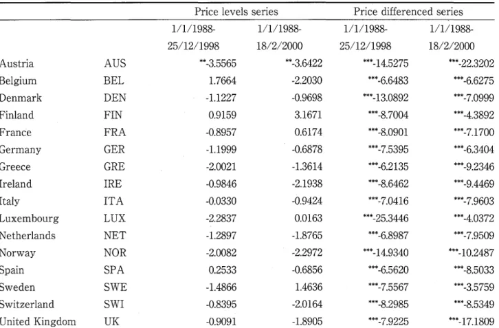
(10) 88. TABLE 1. Augmented Dickey-Fuller (ADF) unit root tests ' differenced series Price. Price levels series. 1/1/1988-. 1/1/1988-. 1/1/1988-. 1/1/1988-. 25/12/1998. 18/2/2000. 25/12/1998. 18/2/2000. Austria. AUS. "*-3.5565. "*-3.6422. ***-14.5275. "**-22.3202. Belgium. BEL. 1.7664. -2.2030. ***-6.6483. ***-6.6275. Denmark. DEN. -1.1227. -O.9698. ***-13.0892. ***-7.0999. Finland. FIN. O.9159. 3.1671. "*"-8.7004. ***-4.3892. FranCe. FRA. -O.8957. O.6174. """-8.0901. ***-7.1700. Germany. -1.1999. -O.6878. ***-7.5395. ***-6.3404. Greece. GER GRE. -2.0021. -1.3614. ***-6.2135. *""-9.2346. Ireland. IRE. -O.9846. -2.1938. "*"-8.6462. ***-9.4469. Italy. ITA. -O.0330. -O.9424. "'-7.0416. ***-7.9603. Luxembourg. -2.2837. O.O163. ***-25.3446. ***-4.0372. -1.2897. -1.8765. ***-6.8987. ***-7.9509. Norway. LUX NET NOR. -2.0082. -2.2972. ***-14.9340. "**-10.2487. Spain. SPA. O.2533. -O.6856. ***-6.5620. ***-8.5033. Sweden. SWE. -1.4866. 1.4636. *""-7.5567. ***-3.5759. Switzerland. SWI. -O.8395. -2.0164. ***-8.2985. ***-8.5349. United Kingdom. UK. -O.9091. -1.8905. ***-7.9225. "*"-17.1809. Netherlands. Notes: Hypotheses Ho: unit root, Hi: no unit root (stationary); the lag orders in the ADF equations are determined by the significance of the coefficient for the lagged terms; for the price Ievels series, intercepts and tends are included, critidal values at the .Ol, .05 and .10 percent level are -3.98, -3.42 and -3.13, respectively; for the price differenced series only intercepts are included, critical values at the .Ol, .05 and .10 percent level are -3.44, -2.87 and -2.57, respectively; asterisks denote significance at the ""* - .Ol, '" m .05 and " - .10 percent level.. chain to be evaluated. However, decomposition of the variance of forecast errors of a given market allows the relative importance of the variance markets in causing fluctuations in that. market to be ascertained.'The decomposition process therefore allows the Variance of the forecast errors to be divided into percentages attributable to innovations in all other markets and. a percentage. attributable to innovations in the given market. ,One problem here is that the decomposition of variances is sensitive to the assumed origin of the shock and to the order it is. transmitted to other markets. To overcome this problem, a generalised impulse response analysis, which is not subject to any arbitrary othogonalisations of innovations in the system, is applied (Masih and Masih 1999).. IV, EMPIRICAL RESULTS Table 1 presents the ADF unit root tests (1) for the sixteen European equity indices in price. level and price-differenced forms. The first column for each form presents tests carried out for period 1/1/1988 to 25/12/1999 (prior to the introduction of the single currency) while the second column details the tests results for the longer period 1/1/1988 to 18/2/2000. In both instances, the.

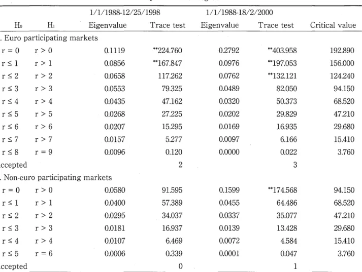
(11) 8g). TABLE 2s. Johansen cointegration tests. 1/1/1988-18/2/2000. 1/1/1988-12/25/1998 Ho. H,. Eigenvalue Tracetest. Eigenvalue Tracetest. Critical value. A. Euro participating markets. r =O. rSl rS2 rS3 rS4 rS5 rS6 rg7 rg8. r>O r>1 r>2 r>3 r>4 r>5 r>6 r>7 r=9. O.1119. *'. 224.760. O.2792. "*. 403.958. 192.890. O.0856. *" 167.847. O.0976. *". 197.053. 156.000. O.0658. 117.262. O.0762. "*. 132.121. 124.240. O.0553. 79.325. O.0489. 82.050. 94.150. O.0435. 47.162. O.0320. 50.373. 68.520. O.0268. 27.225. O.0202. 29.829. 47.210. O.0207. 15.295. O.O169. 16935. 29.680. O.Ol57. 5.277. O.O097. 6.166. 15.410. O.O096. O.120. o.oooo. O.022. 3.760. Accepted. 2. 3. B. Non-euro participating markets. r=O rSl rS2 rS3 rS4. r>O r>1 r>2 r>3 r>4. O.0580 O.0400 O.0295 O.O181 O.OI07. rg5r=6 'O.OO06 Accepted. 91.595. O.1599. 57.389. 174.568. 94.150. O.0455. 64.486. 68.520. 34.037. O.0337. 35.077. 47.210. 16.937. O.O139. 13.428. 29.680. 6.469. O.O072. 4.584. 15.410. O.339. O.OOOI. O.047. 3.760. o. **. 1. Notes: Group A - Includes Belgium, Finland, France, Germany, Ireland, Italy, Luxembourg, Netherlands and Spain (Austria and Portugal are excluded because of stationarity and insufficient data, respectively); Group B m Greece, Norway, Sweden, Switzerland, Denmark and United Kingdom; .05 percent level critical values from OsterwaldLenum (1992); the optimal lag order of each VAR modei was selected using LR tests for the significance of the coefficient for maximum lags and Schwarz's Bayseian Information Criterion; in each cointegrating equation, the intercept (no trend) is included.. null hypothesis of nonstationarity is tested. Analysis of the price levels series indicates nonstationarity for all markets except Austria in both sample periods. However, all of the ADF tests statistics are significant in differenced form, indicating stationarity and the suggestion that each index series (other than Austria) is integrated of order 1 or I(1). The finding of non-stationarity in. levels and stationarity in first differences provides comparable European evidence to Arshanapalli and Doukas (1993), Leachman and Francis (1995), Malliaris and Urrutia (1996) and Kanas (1998), amongst others.. Johansen cointegration tests are used in order to obtain the cointegration rank. Eigenvalues and trace test (3) statistics are detailed in Table 2 for the various null and alternative hypotheses.. As multivariate cointegration tests the results cover each set of markets (ie. euro and non-euro participating) rather than simple bivariate combinations. They therefore consider the wide range of portfolio diversification options available to non-European investors, as well as the scope of. financial integration that may not be reflected in pairwise combinations. Two sets of tests are.

(12) 9o included. The first group of tests corresponds to the nine markets that participated in the single currency [Austria is not included because it is of order I(O), while insufficient data existed to construct the tests for Portugal]. Critical values for these statistics are obtained from Osterwald-. Lenum (1992) and are detailed in the final column of Table 2. In terms of euro-participating markets, and for the period up until the adoption of the single currency, both trace tests statistics are greater than the critical value for the null hypotheses of r. == O and r S{ 1 thereby rejecting the null hypothesis in both cases. However, in the period up until the adoption of the single currency the null hypothesis of r S 2 fails to be rejected in favour r > 2. indicating the order of cointegration is 2. In the time series including the period since the adoption of the single currency, similar hypothesis are rejected up to, but not including, r g 3 suggesting an order of integration of 3.. The primary finding is that there is a stationary long-run relationship between the equity markets of the euro-currency area and that the number of long-run cointegrating relationships among euro-participating markets has increased when the period including the adoption of the single currency is analysed. Johansen and Juselius (1993) also point out that larger eigenvalues. are associated with the cointegrating vector being more correlated with the stationary component of the underlying process, and therefore are suggestive of the relative strength of the. long run relationship. For both sets of markets (ie. euro and non-euro participating) the eigenvalues are larger when the period since the adoption of the single currency is included. Together, these suggest that the level of long-run financial integration among these markets has intensified. However, this result must be taken ･in context. The finding of a cointegrating vector. across indices demonstrates that across the sample the markets have moved together in an equilibrium relationship. It does not mean, however, that there have not been sub-periods during. which the indices have moved apart. For the non-euro participating economies in Table 2 the null hypothesis of r = O fails to be rejected in the period befo're the final of EMU, thereby suggesting that there is no long term cointegration for these indices. However, in period including the period since the final stage of EMU the null hypothesis of r S cannot be rejected suggesting an order of cointegration of 1. The. suggestion in this case, is that no stationary long-run relationship existed between non-euro participating economies prior to the introduction of the single currency, but that a long-run relationship has been established when the final stage of EMU is included.. Since cointegration exists between both sets of indices, that is, euro and non-euro participating markets, the Granger causality tests are performed on the basis of equation (5). F: statistics are calculated to test the null hypothesis that the first index series does not Granger. cause the second, against the alternative hypothesis that the first index Granger causes the second. Calculated statistics and p-values for the euro-participating markets are detailed in Table 3. Because the Austrian market was found to be stationary in levels, that is I(O), it is included in. the Granger causality test procedure in levels, while all other markets are specified in first. differences. The first matrix of test statistics in Table 3 relates to the period 1/1/1988 to 25/12/1998. Among the ten participating markets (excluding Portugal) nineteen significant causal links are found (at the .10 level or lower), For example, column 2 shows that the French, Finnish,.

(13) 9I. TABLE 3.. Granger causality tests for euro participating markets, 1/1/1988 - 18/2/2000. Period 1/1/1988 - 12/25/1998. Market AUS AUS BEL FIN. FRA GER IRE. ITA. LUX. NET SPA. BEL. FIN. FRA. GER. IRE. ITA. LUX. NET. SPA. Causes. 5.8649. 1.7013. 1.0603. 1.2634. 2.9062. O.5924. 1.0413. O.5759. 1.2918. 2. (O.O158). (O.1927). (O.3036). (O.0888). (O.4418). (O.3080). (O.4483). (O.2562). O.OO05. 10.9889. O.3502. (02615) 3.9604. O.2223. O.0866. O.5761. 2.6885. 2.8547. (O.9813). (O.OOIO). (O.5543). (O.0471). (O.6375). (O.7687). (O.4482). (O.1016). (O.0917) (O.1987). O.OOOO 14.8890. 1.4656. 5.6638. O.1455. 4.1913. 2.5117. (1.0000) (O.OOOI). (O.2265). (O.O177). (O.7030). (O.0411). (O.1136). 5.4148 5.5820. O.OO09. 11.5036. O.1331. O.0741. 8.0692. O.3344 (05633) 2.9398. (O.0203) (O.O185). (O.9762). (O.OO07). (O.7154). (O.7855). (O.O047). (O.0870). (O.0444) (O.9742) (O.8528). O.6244 O.7484. O.5065. O.1272. O.3587. 1.3542. O.2144. (O.4297) (O.3874). (O.4770). (O.7214). (O.5494). (O.2450>. (O.6435). 1.8068 1.5042. 1.2648. l.2963. 2.0649. O.9393. O.1696. O.0584 (08092) O.1364. (O.1794) (O.2205). (O.2612). (O.2554). (O.1513). (O.3329). (O.6806). (O.7121). 1.6559 4.0611. O.OOIO O.0344. O.8390 O.0269. O.0410. O.9028. O.2109. 2.0515. O.2426. O.2385. O.6050. (O.3601) (O.8698). (O.8395). (O.3424). (O.6463). (O.1526). (O.6225). (O.6255). (O.4370). l.O053. O.1137. 2.8627 1.4432. O.8082. O.4186. 4.6707. O.1257. O.3792. (OD912) (O.2301). (O.3690). (O.5179). (O.0311). (O.7230). (O.5383). O.8813 O.OOOI. 2.9632. O.1409. O.6552. O.4414. O.1219. O.0613. O.7979. (O.0857). (O.7075). (O.4186). (O.5067). (O.7271). (O.8046). (O.3721). O.1533 O.5615. 1.5953. O.3276. 2.9906. 7.0972. 2.3334. O.1798. O.8425. (O.6956) (O.4540). (O.2071). (O.5673). (O.0843). (O.O079). (O.1272). (O.6717). (O.3591). 2. o. 5. 2. 1. 1. 1. 23. 3. 6 o o. o 2. (O.3165). (O.7361). (O.3483) (O.9914). Caused. 3. ･1. 2 2. 19. Period 1/1/1988 - 18/2/2000. AUS BEL FIN. FRA GER IRE. ITA. LUX. NET SPA Caused. AUS. BEL. FIN. FRA. GER. IRE. ITA. LUX. NET. SPA. Causes. 1.1451. O.0244. 1.3800. O.9805. 1.4670. O.1010. ID504. O.7146. 1.4344. o. (O.2850). (O.8760). (O.2405). (O.3225). (O.2263). (O.7508). (O.3058). (O.3982). (O.2315). O.3422. 4.9196. 1.2814. 2.3223. O.0885. O.1587. 6.6202. 2.3034. 1.8552. (O.5588). (O.0269). (O.2581). (O.1280). (O.7662). (O.6905). (O.OI03). (O.1296). (O.1737). O.6427. O.0939. O.1052. 7.3453. O.1905. 2.8695. 2.1791. 1.5939. 1.8349. (O.7457). (O.O069). (O.6627). (O.0908). (O.1404). (O.2072). (O.1760). 2 2. (O.4230). (O.7594). 52111. 4.5432. 4.8699. 7.1181. O.2928. O.1883. O.8173. I.5578. 6.4132. (O.0228). (O.0334). (O.0277). (O.O078). (O.5886). (O.6645). (O.3663). (O.2125). (O.Ol16). o.oooo･. O.0657. O.6780. O.0675. O.1236. O.0328. O.5645. O.OO05. 4.6229. (O.9959). (O.7978). (O.4106). (O.7952). (O.7253). (O.8564). (O.4527). (O.9820). (O.0319). O.2384. O.4143. O.3l64. O.3426. (O.6256). (O.5586). 1.1434. 4.5523. 1.2144. O.0954. O.7176. (O.2854). (O.0333). (O.2709). (O.7576). (O.3973). (O.5200). (O.5740). O.4661. O.2062. O.1629. 1.9655. O.0243. 1.4130. O.1926. O.l284. O.8922. (O.4951). (O.6499). (O.6866). (O.1614). (O.8762). (O.2350). (O.6609). (O.7202). (O.3453). OD181. 4.2143. 5.2163. O.2981. O.0603. 1.8182. 1.9409. O.O194. 2.4306. (O.8930). (O.0405). (O.0227). (O.5853). (O.8061). <O.1780). (O.1641). (O.8892). (O.1195). O.O020. O.2126. 2.0809. O.5819. O.5180. O.0209. O.O075. 1.1332. O.2535. (O.9644). (O.6449). (O.1497). (O.4459). (O.4720). (O.8852). (O.9312). (O.2875). (O.6148). O.2075. O.2030. 2.8427. O.3171. O.4662. 5.5288. 3.2022. O.1574. O.3972. (O.6489). (O.6524). (O.0923). (O.5736). (O.4950). (O.O190). (O.0740). (O.6917). (O.5288). 1. 4. 4. o. 2. 1. l. 1. o. 5 1. 1. o 2. o 3. 2. 16. Notes: Granger causality tests are conducted by adjusting the long-term cointegrating relationship by the ECM; figures in brackets are p-values; tests indicate Granger causality by row to column and Granger caused by column to row, for example, in the period 1/1/1988 - 18/2/2000 France (row) Granger causes five markets (AUS, BEL, FIN, GER and SPA) but is not Granger caused by any markets (using a critical value of .10); levels data is used in the ECM for Austria because of stationarity..

(14) 92. Luxembourgian and Belgian markets affect the Austrian market; the Irish market (column 6) is influenced by Spain and Austria; and France influences the Netherlands market (column 9).. Further insights are gained by examining the rows in Table 3 indicating the effects of a particular market on all markets. It is evident that the French market is the most influential. market in the single currency area, influencing Austria, Belgium, Germany, Luxembourg, Netherlands and Spain. In a similar cointegration approach, Friedman and Shachmurove (1997) also found that France affected the Belgian and German markets, while Meric and Meric (1997). established high pairwise correlations between France and Germany, Belgium and the Netherlands, though using a correlation approach. The least influential markets in terms of Granger-causality include Ireland, Germany and Italy. There is also an indication that there is. feedback at play in several pairwise combinations: for example, Belgium Granger-causes Finland. and Finland Granger-causes Belgium. The second set of test statistics and p-values in Table 3 relates to the period including the. third and final stage of EMU. The results in this sample period are broadly comparable to those found earlier with France being the market that Granger causes most other indices. While there is a small fall in the number of short-run causal links (from nineteen to sixteen), it is thought that. the process of economic convergence that extends over much of the sample period already. encompasses most of the changes brought about by the adoption of the single currency. However, caution should also be exercised in interpreting the fall in causal links since they reflect. only the most direct causal linkage, and not the indirect influences from markets flowing through other markets, This is just one benefit of examining the variance decomposition as presented in. Table 5. 0ne implication of the results in Table 3, however, is that there may be no gains from pairwise portfolio diversification between those countries where a significant causal relationship. exists. Also since we have a finding of causality these markets must be seen as violating weak-. form efficiency since one of the markets can help forecast the other. In all other cases, the absence of Granger causality implies that there are sufficient short-run differences between the markets for non-European investors to gain by portfolio diversification.. Table 4 presents a similar analysis for the six equity markets that chose not to or could not. participate in the single currency. All of these markets are also members of the EU with the exception of Norway and Switzerland. In the period leading up to the final stage of EMU there. are eleven short-run causal relationships among these economies. For example, Switzerland Granger causes Greece and Sweden at the .Ol level, the United Kingdom at the .05 level and Norway at the .10 Ievel. Correspondingly, Sweden is Granger caused by Greece at the ,05 level and Switzerland and the United Kingdom at the .Ol level. In the period including the third and. final stage of EMU the number of short-run causal relationships among these markets has increased to sixteen. The U.K. and Switzerland are still the markets that are most influential in. term of the remaining markets. For example, Switzerland Granger causes Norway at the .10 level, Denmark at the .05 level and all remaining markets at the Ol leveL.

(15) 93. TABLE 4. Granger causality tests for non-euro participating markets. Period 1/1/1988 - 25/12/1998. Market. SWE. SWI. O.1760. 4.7362. 1.8603. 1.1558 ll5902. (O.6750). (O.0299). (O.1731). (02828) (O.2078). 2.4849. OD471. O.0661. 1.1289 O.0676. (O.1155). (O.8282). (O.7972). (O.2885) (O.7950). GRE. NOR. SWE SWI. DEN. UK Caused. DEN UK. NOR. GRE. Causes. 1 o. 1.9740. O.8491. 12.9403. 2.1314 3.l374. (O.1606). (O.3572). (O.OO03). (O.1449) (O.0771). 8.3400. 2.8844. 32.7384. 1.6770 5.6701. (O.O040). (O.0900). (o.oooo). (O.1958) (O.O176). O.5068. O.3082. 1.2783. O.2871. O.0366. (O.4768). (O.5790). (O.2587). (O.5923). (O.8484). O.6588. 10.8216. 20.8338. 6.7633. 25.3819. (O.4173). (O.OOII). (o.oooo). (O.O095). (o.oooo). 1. 2. 3. 2. 1. NOR. SWE. SWI. DEN UK. Causes. 1.4212. 16.1255. 9.2572. 1.6613 19.7781. 3. (O.2337). (O.OOOI). (O.O024). (O.1979) (O.OOOO). 3.5106. O.3814. O.5218. 1.8535 O.O175. (O.0614). (O.5371). (O.4703). (O.1739) (O.8949). 2. 4. o. 4. 2. 11. Period 1/1/1988 - 18/2/2000. GRE. GRE. NOR. SWE SWI. DEN UK Caused. 3.5070. 3.1543. 8.6256. O.4650 1.1471. (O.0616). (O.0762). (O.O034). (O.4956) (O.2846). 9.0867. 3.6682. 21.6388. 4.2675 9.4080. (O.O027). (O.0559). (o.oooo). (O.0393) (O.O023>. O.1531. O.Ol16. O.7481. O.3625. O.O067. (O.6957). (O.9143). (O.3874). (O.5473). (O.9349). 3.0290. 11.8902. 2.6908. 9.1096. 16.1923. (O.0823). (O.OO06). (O.IO14). (O.O026). (O.OOOI). 4. 3. 2. 3. 2. 1. 3. 5. o. 4. 2. l6. Notes: Granger causality tests are conducted by adjusting the long-term cointegrating relationship by the ECM; figures in brackets are p-values; tests indicate Granger causality by row to col.umn and Granger caused by column to row, for example, in the period 1/1/1988 - 18/2/2000 the U.K. (row). Granger causes four markets (GRE, NOR, SWI and DEN) and is Granger caused by Greece and Switzerland (using a critical value of .10)..

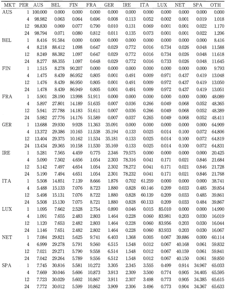
(16) 94. TABLE 5.. Generalised variance decomposition for euro participating markets, 1/1/1988 - 18/2/2000. MKT PER AUS. AUS. BEL. FIN. FRA. GER. IRE. ITA. LUX. NET. SPA. BEL. FIN. FRA. GER. IRE. ITA. LUX. NET. SPA. OTH. 1. 100.000. o.ooo. o.ooo. o.ooo. o.ooo. o.ooo. o.ooo. o.ooo. o.ooo. o.ooo. o.ooo. 4. 98.982. O.063. O.064. O.696. O.O08. O.113. O.052. O.O02. O.OOI. O.O19. 1.018. 12. 98.830. O.069. O.077. O.790. O.OIO. O.131. O.069. ODOI. O.OOI. O.022. 1.170. 24. 98.794. O.071. O.080. O.812. O.Oll. O.135. O.073. O.OOI. O.OOI. O.022. 1.206. 1. 8.416. 91.584. o.ooo. o.ooo. o.ooo. o.ooo. o.ooo. o.ooo. o.ooo. o.ooo. 8.416. 4. 8.218. 88.412. 1.098. O.647. O.029. O.772. OO16. O.734. O.026. O.048. 11.588. 12. 8.249. 88.382. 1.097. O.647. O.029. O.772. O.O16. O.734. O.026. O.048. 11.618. 24. 8.277. 88.355. 1.097. O.648. O.029. O.772. O.O16. O.733. O.026. O.048.. 11.645. 1. l.515. 8.278. 90.207. o.ooo. o.ooo. o.ooo. o.ooo. o.ooo. o.ooo. o.ooo. 9.793. 4. 1.475. 8.439. 86.952. O.805. O.OOI. ･O.491. O.O09. -O.971. O.437. O.419. 13.048. 12. 1.476. 8.439. 86.950. O.805. O.OOI. O.491. O.O09. O.972. O.437. O.419. 13.050. 24. 1.478. 8.439. 86.949. O.805. O.OOI. O.491. O.O09. O.972. O.437. O.419. 13.051. 1. 5.901. 28.190. 13.998. 51.911. o.ooo. o.ooo. o.ooo. o.ooo. o.ooo. o.ooo. 48.089. 4. 5.897. 27.801. 14.189. 51.635. O.O07. O.036. O.266. O.049. O.068. O.052. 48.365. 12. 5.941. 27.788. 14.183. 5L611. O.O07. O.036. O.266. O.049. O.068. O.052. 48.389. 24. 5.982. 27.776･. 14.176. 51.589. O.O07. O.037. O.265. O.049. O.068. O.052. 48.411. 1. 13.688. 29.930. 9.928. 11.363. 35.091. o.ooo. o.ooo. o.ooo. o.ooo. o.ooo. 64.909. 4. 13.372. 29.386. 1O.165. 11.538. 35.194. O.133. O.025. O.O14. O.100. O.072. 64.806. 12. 13.404. 29.375. 10.162. ll.534. 35.181. O.133. O.025. O.O14'. O.100. O.072,. 64.819. 24. 13.434. 29.365. 10.158. 11.530. 35.169. O.133. O.025. O.O14. O.100. O.072. 64.831. 1. 5281. 7.565. 4.459. O.775. 2.346. -79.575. o.ooo. o.ooo. o.ooo. o.ooo. 20.425. 4. 5.090. 7.502. 4.656. 1.054. 2.303. 78.316. O.041. O.171. O.021. O.846. 21.684. 12. 5.142. 7.497. 4.654. 1.054. 2.302. 78.272. O.041. O.171. O.021. O.846. 21.728. 24. 5.190. 7.494. 4.651. 1.054. 2.301. 78.232. O.041. O.171. O.021. O.846. 21.768-. 1. 5.508. 14.851. 7.139. 8.666. 1.876. O.702. 61.259. o.ooo. o.ooo. o.ooo. 38.741. 4. 5.488. 15.133. 7.076. 8.723. 1.880. O.828. 60.146. O.209. O.033. O.485. 39.854. 12. 5.498. 15.131. 7.076. 8.722. 1.880. O.828. .60.139. O.209. O.033. O.485. 39.861. 24. 5.508. 15.130. 7.075. 8.721. 1.880. O.828. 60.133. O.209. O.033. O.484. 39.867. 1. 1.095. 7.662. 2.528. 2.754. O.890. O.046. O.O15. 85.010. o.ooo. o.ooo. 14.990. 4. 1.091. 7.655. 2.483. 1.464. O.228. O.060. 83.981. O.203. O.030. 16.019. 12. 1.120. 7.653. 2.482. 2.803 2.8o3. 1.464. O.228. O.060. 83.956. O.203. O.030. 16.044. 24. 1.146. 7.651. 2.482. 2.802. 1A64. O.228. O.060. 83.933. O.203. O.030. 16.067. 1. 7.084. 29.821. 5.625. 9.741. 6.403. 1.368. O.O05. O.067. 39.886. o.ooo. 60.114. 4. 6.999. 29.278. 5.791. 9.560. 6.515. 1.548. O.O12. O.067. 40.168. O061. 59.832. 12. 7.021. 29271. 5.790. 9.558. 6.514. 1.548. O.O12. O.067. 40.159. O.061. 59.841. 24. 7.042. 29.264. 5.789. 9.556. 6.512. 1.548. O.O12. O.067. 40.150. O.061. 59.850. 1. 7.745. 30.816. 5.581. 10272. 3.305. 2.345. 3.555. O.499. 0914. 34.967. 65.033. 4. 7.669. 30.046. 5.606. IO.873. 3.913. 2.309. 3.500. O.774. O.905. 34.405. 65.595. 12. 7.723. 30.029. 5.602. 10.867. 3.911. 2.307. 3.498. O.773. O.905. 34.385. 65.615. 24. 7.772. 30.012. 5.599. 10.862. 3.909. 2.306. 3.496. O.773. O.904. 34.367. 65.633. Notes: The decomposition order is indicated by column; the final column (OTH) is the percentage of forecast error variance of the market indicated in first column (MKT) explained by all other markets except the market's own innovations; the periods (PER) in the second column are in weeks..

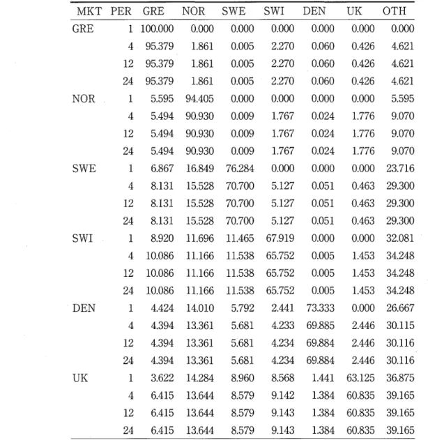
(17) 9S Interesting, we find evidence for Granger causality at the .10 level of significarice or lower for sixteen out of the thirty-six possible relationships in the sample. In many of these cases, a mutual. relationship can be observed As expected, the U.K. and Switzerland are the most influential markets in this sample, with the U.K. Granger causing four markets and Switzerland five. The dominant position of these markets, one being a non-EU member and the other a non-participant in the single currency, appears to have been unchanged in the period before and after the final. stage of EMU. Table 5 presents the decomposition of the forecast error variance for 1-week, 4-week, 12week and 24-week ahead horizons for euro participating markets over the entire sample period. Each row indicates the percentage of forecast error variance explained by the column heading for the market indicated in the first column. At the 1-week horizon, the variance in the Austrian. market is completely explained by its own innovations, whereas in the remaining markets some percentage of variance is explained by innovations in other markets. For example, other markets explain 8.4 percent of variance in the Belgian market, 9.8 for Finland, 48.1 for France, 64.9 for Germany, 20.4 for Ireland, 38.7 for Italy, 15.1 for Luxembourg, 60.1 for the Netherlands and 65 for Spain. These would indicate that the Belgian market' is the least influenced by innovation in other Markets, while the Spanish market is the most sensitive.. The evidence presented also reinforces the suggestion many smaller markets in the euro currency area are relatively isolated, and therefore prospects for international diversification still. exist. Markets least explained by innovations in other markets include Austria, Belgium, Finland, Ireland and Luxembourg. This effect also appears to persist for considerable periods of time. The results are also interesting in that they illuminate aspects of market interaction not indicated by. the Granger causality tests. A notable example is the apparent dominance of France in Grangercausing five other euro-participating markets in this sample period. In the forecast variance. decomposition of analysis, the French market still significantly influences other markets, especially Germany, Italy and Spain, but the variance explained for Ireland, Belgium, Finland and Austria is less than one percent.. Table 6 details the results of a similar analysis conducted for the six non-euro participating. markets. Once again, small markets such as Greece and Norway are least explained by variations in other markets (O and 4.6 percent, respectively). Other markets explain some 23 percent of the variance in the Swedish market, 32 percent of the Swiss, 27 percent of Danish, and 37 percent of. the U.K. market after a one-week period. There is also generally a stronger interrelationship. among the four members of the EU, though the variance in the Greek market is still very much unexplained by variations in the other markets.. V. CONCLUDING REMARKS This paper investigates long-term and short-term relationshiPs among sixteen European equity markets during the period 1988 to 2000. Eleven of these markets are participants in the third and final stage of EMU (the adoption of a single currency) while four of the five remaining. markets are non-euro participating Member States of the EU. Multivariate cointegrating techniques are used to establish long-term relationships among these markets and Granger.

(18) g6. TABLE 6.. Generalised variance decomposition for non-euro participating markets, 1/1/1988 - 18/2/2000. MKT PER GRE GRE. NOR. SWE. SWI. DEN. UK. 1. 100.000. NOR SWE. SWI. DEN. o.ooo. o.ooo. o.ooo. o.ooo. UK. OTH. o.ooo. o.ooo. 4. 95.379.. 1.861. O.O05. 2.270. O.060. O.426. 4.621. 12. 95.379. 1.861. O.O05. 2.270. O.060. O.426. 4.621. 24. 95.379. 1.861. O.O05. 2.270. O.060. O.426. 4.621. 1. 5.595. 94.405. o.ooo. o.ooo. o.ooo. o.ooo. 5.595. 4. 5.494. 90.930. O.O09. 1.767. O.024. 1.776. 9.070. 12. 5.494. 90.930. O.O09. 1.767. O.024. 1.776. 9.070. 24. 5.494. 90.930. O.O09. 1.767. O.024. 1.776. 9070. 1. 6.867. 16.849. 76.284. o.ooo. o.ooo. o.ooo. 23.716. 4. 8.131. 15.528. 70.700. 5.127. O.051. O.463. 29.300. 12. 8.131. 15.528. 70.700. 5.127. O.051. O.463. 29.300. 24. 8.131. 15.528. 70.700. 5.127. O.051. O.463. 29.300. 1. 8.920. 11.696. 11.465. 67919. o.ooo. o.ooo. 32081. 4. 10.086. 11.166. 11.538. 65.752. O.O05. 1.453. 34.248. 12. 10.086. IL166. 11.538. 65.752. O.O05. 1.453. 34.248. 24. 10.086. 11.166. 11.538. 65.752. O.O05. 1.453. 34.248. 1. 4.424. 14.010. 5.792. 2.441. 73.333. o:ooo. 26.667. 4. 4.394. 13.361. 5.681. 4.233. 69.885. 2.446. 30.115. 12. 4.394. 13.361. 51681. 4.234. 69.884. 2.446. 30.116. 24. 4.394. 13.361. 5.681. 4.234. 69.884. 2.446. 1. 3.622. 14.284. 8.960. 8.568. 1.441. 63.125. 36.875. 4. 6.415. 13.644. 8.579. 9.142. 1.384. 60.835. 39.165. 12. 6.415. 13.644. 8.579. 9.143. 1.384. 60.835. 39.165. 24. 6.415. 13.644. 8.579. 9.143. 1.384. 60.835. 39.165. 30.116'. Notes: The decomposition order is indicated by column; the final column (OTH) is the percentage of forecast error variance of the market indicated in first column (MKT) explained by all other markets except the market's own innovations; the periods (PER> in the second column are in weeks.. caudsality tests are used to measure causal relationships in the short-term within an error correcting model (ECM).. The results indicate, as expected, that the Euro-11 equity markets are highly integrated,. both before and after the transition to the single currency. This long-term interdependency appear to be unaffected by the actual transition to the euro on 1 January 1999, albeit within a short sample period, and is indicative of the decade-long process of economic convergence spelt out in the 1992 Maastricht Treaty. Broad structural and institutional changes, along convergence. criteria aimed at achieving a high degree of sustainable economic convergence have ensured. developments in the European monetary sector has gone far towards quickening the pace of. overall financial integration. '.

(19) 97 However, the level of financial integration within non-euro participating Member States and. non-EU members has also increased over this period, especially when considering the period after the introduction of the single currency. Justification for this is not hard to find, especially. since five of these markets are also Member States of the EU. Likewise, it has been known for. some time that the U.K. and Denmark would not move to the final stage of EMU on 1 January. 1999, and that Greece and Sweden did not participate in the ERM in the two years ending February 1998 (as per the required convergence criteria). Accordingly, as markets not bound by. the framework necessary for the conduct of economic policy in the euro area these mostly EU economies have just as much in common as the actual participants.. The findings obtained in this paper have obvious implications for the purported benefits of international portfolio diversification among the several European equity markets. In effect, the. strong short-term causality and long-term linkages among the national markets would indicate. that the returns from such a strategy have diminished markedly. However, while the large equity markets in the U.K., France and Switzerland remain the most influential, the lower causal relationships that exist between these and at least some of the middle-sized (Belgium, Spain and. Netherlands) and smaller (Ireland, Luxembourg, Finland and Norway) equity markets suggests that opportunities for diversification in at least some pairwise combinations may still exist. For. example, France Granger-causes the medium-sized markets of Spain and Belgium and the smaller. sized market of Finland, but there is no direct causal link from France to the Netherlands, Ireland or Luxembourg. This is further reinforced by the results of a decomposition of variance analysis that indicates that a distinguishing characteristic of most of the smaller markets is the. extremely low level of variance explained by other markets. For example, even among the europarticipating markets other markets explain less than ten percent of the variance in Austria, Belgium and Finland.. REFERENCES Abbot, A.B. and Chow, K.V. (1993) Cointegration among European equity markets, Journal of Mulimational FYnancial MRnagement 2(3-4), 167-184.. Akdogan, H. (1995) The Integration of Jhternational Capital Markets: Theory and Empin'cai Evidence, Edward Elgar, Aldershot. Arshanapalli, B. and Doukas, J. (1993) International stock market linkages: Evidence from the preand post-October 1987 period, fournal of Banking and Finance, 17(1), 193-208.. Cheung, Y.W. and Lai, K.S. (1999) Macroeconomic determinants of Iong-term stock market comovements among major EMS countries, Applied Financial Economics, 9(1), 73-85.. Commission of the European Communities (1997) Econoniic and Monetary Ubion: External Aspects of EMU Commission Working Document, SEC(97) 699, WWW site accessed 6 March 1999. <http://europa.eu.int/scadplus/leg/en/lvb/125032.htm>. Commission of the European Communities (1999) 1999 Annual Economic Report, The EU Economy at the Arrival of the Euro: Promoting Growth, Employmellt and Stability, Brussels. Darbar, S.M. and Deb, P. (1997) Co-movement in international equity markets, fournal of lZinancial.

(20) 98. Research, 20(3), 305-322.. Elyasiani, E. Perera, P. and Puri, T.N. (1998) Interdependence and dynamic linkages between stock markets of Sri Lanka and its trading partners, Journal of Multinational Financial. imnagement 8(1), 89-101. Engle, R. F. and Granger, C.W.J. (1987) Co-integration and Error Correction: Representation, Estimation, and Testing, Econometn'ca, 55(2), 251-276.. Espitia. M. and Santamaria, R (1994) International diversification among the capital markets of the EEC, Applied Financial Economics, 4(1), 1-10.. Francis, B.B. and Leachman, L.L (1998) Superexogeneity and the dynamic linkages among international equity markets, Journal ofinternational Money and Einance, 17(4), 475-492.. Friedman, J. and Sgachmurove, Y. (1997) Co-movements of major European community stock markets: A vector autoregression analysis, GIobal Finance Journal, 8(2), 257-277.. Gallagher, L. (1995) Interdependencies among the Irish, British and German stock markets, Economic and Social Review; 26(2), 131-147. Granger, C. W. J, (1969) Investigating causal relations by econometric models and cross-spectral methods, Econometizica, 37(3), 424-438.. Hanna, M.E. McCormack, J.P..and Perdue, G. (1999) A nineties perspective on international diversification, IZinancial Servi'ces Reviev￠ 8(1), 37-45.. Johansen, S. (1991) Estimation and hypothesis testing of cointegration vectors in Gaussian vector. autoregressive models, Econometrica, 59(6), 1551-1580.. Johansen, S. and K. Juselius (1990) Maximum likelihood estimation and inferences on cointegration - with applications to the demand for money, Oxford BuUetin of Economics and Statistics, 52(2), 169-210.. Kanas, A. (1998) Linkages between the US and European equity markets: Further evidence from cointegration tests, Applied 1[nyinancial Economics, 8(6), 607-614.. Kwan, A.C.C. Sim, AB. and Cotsomitis, J.A. (1995) The causal relationships between equity indices. on world exchanges, Applied Economics, 27(1), 33-27.. Leachman, L.L. and Francis, B. (1995) Long-run relations among the G-5 and G-7 equity markets: Evidence on the Plaza and Louvre Accords, Journal of lVlacroeconomics, 17(4), 551-577.. Levy, H. and Sarnat, M. (1970) International portfolio diversification of investment portfolios,. American Economic Reviev￠ 60(3), 668-675. Longin, F. and Solnik, B. (1995) Is the correlation in international equity returns constant: 19601990?, Journal of international Money and Einance, 14(1), 3-26.. MacKinnon, J.G. (1991) Critical Values for Cointegration Tests, in R.F.Engle and C,WJ. Granger. (eds.) Long-run Economic Relationships: Readings ifl Cointegration, 267-276, Oxford University Press, New York. Malliaris, A.G. and Urrutia, J.L (1996) European stock market fluctuations: Short and long term links, fouznal oflnternational Financial A(lar:kets, Institutions and MoneM 6(2-3), 21-33.. Meric, I. and Meric, G. 1997) Co-movements of European equity markets before and after the 1987 Crash, Multinational finance fournal, 1(2), 137-152.. Osterwald-Lenum, M. (1992), Note with quantiles of the asymptotic distribution of the maximum.

(21) 99 likelihood cointegration rank.test statistics, Oxford Bulletin of Ecollomics and Statistics, 54(3), 461-72.. Ramchand, L. and SusmeL R. (1998) Volatility and cross-correlation across major stock markets, Jburnal of Empin'cal Finance, 5(4), 397-416.. Richards, AJ. (1995) Comovements in national stock market returns: Evidence of predictability, but not cointegration, fournal of Molletary Economics, 36(3), 631-654.. Roca, ED. (1999) Short-term and long-term price linkages between the equity markets of Australia and its major trading partners, Applied Financial Economics, 9(5), 501-511.. Shawky, H.A. KuenzeL R. and Mikhail, A.D. (1997) International portfolio diversification: A synthesis and an update, Jouznal of international IZinancial INdarkets, 7(4), 303-327.. Solnik, B. (1974) Why not diversify internationally rather than domestically?, 1[nyinallcial Analysts .lburnaL 30(4), 48-54.. Solnik, B. Boucrelle, C. and Le Fur Y. (1996) International market correlation and volatility, Eiflancial Analysts JournaL 52(5), 17-34.. Yuhn, K.H. (1997) Financial integration and market efficiency: Some international evidence from cointegration tests, international Economic .JburnaL 11(2), 103-116.. (Andrew C. Worthington : School of Economics and Finance, Queensland University of Technology, Australia). (Masaki Katsuura 1 Faculty of Economics, Meijo University, Japan). (Helen Higgs : School of Economics and Finance, Queensland University of Technology, Australia).

(22)