DEFAULT RISK OF INDONESIAN GOVERNMENT BOND
52109610
TRIANTO, Edi
DEFAULT RISK OF INDONESIAN GOVERNMENT BOND
Submitted by
TRIANTO, Edi
July 2011
This Thesis is presented to the Higher Degree Committee of
Ritsumeikan Asia Pacific University
in Partial Fulfillments of the Requirements for the Degree of
Master of Business Administration
Abstract
This research is aimed to find an explanation of fluctuation in Indonesian CDS spreads during January 2007 to July 2010. Macroeconomic variables and market sentiment are selected to be used in this analysis. Symmetric Diagonal VECH GARCH model and Granger causality test have been conducted to reveal relationship amongst variables and to select variables will be used in regression analysis. The final model suggests that Indonesian credit risk fluctuation can be explained by variability of exchange rate and global market sentiment. It also suggests that financial shock from developed country is transmitted to Indonesian economy through a direct way, changes in market sentiment, rather than from trade channel.
i
CONTENTS
LIST OF FIGURES iv LIST OF TABLES v CHAPTER I INTRODUCTION 1 1.1 Background 1.2 Research Question 1.3 Research Structure 1 4 5CHAPTER II LITERATURE REVIEW 9
2.1 Default Risk Indicators 2.1.1 Credit Rating
2.1.2 Debt to GDP Ratio 2.1.3 Bond Yield Spreads
2.1.4 Credit Default Swap Spreads
9 9 11 13 14 2.2 Credit Default Swap Market and Mechanism 15 2.3 Determinants of Default Risk and CDS Spreads 16 2.4 CDS Market, Bond Market, and Stock Market
Relationship
21
CHAPTER III VARIABLE CONSIDERATION 24
3.1 Data Level 24 3.2 Macroeconomic Variables 3.2.1 Bond Spreads 3.2.2 US Dollar Rate 3.2.3 Export 3.2.4 Import 3.2.5 Foreign Reserves 3.2.6 Inflation Rate 27 28 28 29 30 30 31 3.3. Market Sentiment, Global or Domestic? 32
ii 3.4 Variable Selection Method
3.4.1 Symmetric Diagonal VECH GARCH Model 3.4.2 Granger Causality Test
33 34 37
3.5 Hypothesis 39
CHAPTER IV DATA AND METHODOLOGY 40
4.1 Data 40
4.2 Methodology
4.2.1 Investigating Daily Data Relationship and Variable Selection Using GARCH Model
4.2.2 Investigating Market Sentiment Role to Indonesian CDS Spreads Using Granger Causality Test
4.2.3 Regression Analysis
42 42
43
44
CHAPTER V INDONESIAN GOVERNMENT BOND 47
5.1 Structure of Indonesian Government Bond
5.2 Domestic and Foreign Currency Denominated Bond Proportion
5.3 Foreign Investor Ownership in Domestic Government Bond
5.4 Debt to GDP Ratio 5.5 Credit Rating History
47 50
53
54 55
CHAPTER VI EMPIRICAL RESULT AND MANAGERIAL INSIGHT 58
6.1 Relationship Amongst Variables Based on GARCH Model
6.2 Granger Causality Test Result 6.3 Regression Analysis Result
6.3.1 Independent Variables : Macroeconomic Variables 6.3.2 Independent Variables : Macroeconomic Variables
and Market Sentiment
58
61 65 66 67
iii
6.3.3 Test of Including Bond Spreads Variable 68
6.4 Managerial Insight 6.4.1 Insignificant Variables
6.4.1.1 Changes in Jakarta Stock Exchange Index 6.4.1.2 Inflation
6.4.1.3 Export
6.4.1.4 Foreign Reserves and Import 6.4.1.5 Bond Spreads
6.4.2 Significant Variables
6.4.2.1 US Dollar Rate and Indonesian Credit Default Risk 6.4.2.2 Changes in Dow Jones Industrial Average Index
and Indonesian Credit Risk 6.4.3 Role of Government 69 70 70 71 73 74 75 75 75 81 84
CHAPTER VII SUMMARY AND CONCLUSION 86
ACKNOWLEDGEMENT 90
iv
LIST OF FIGURES
Figure 1 Indonesian Credit Default Swap Spreads: January 2007- July 2010 (basis points)
4
Figure 2 Proportion of Indonesian Government Bond Issuance 2005-2010 (Trillion Rupiah)
50
Figure 3 Foreign Investor Ownership in Domestic Government Bond (Trillion Rupiah)
54
Figure 4 Indonesian Debt to GDP Ratio 55
Figure 5 Changes of Foreign Investor Ownership in Domestic Bond (Trillion Rupiah)
78
v
LIST OF TABLES
Table 1 Independent Variables Used in Previous Studies 25 Table 2 Indonesian Credit Rating History from 2005 to
July 2010
56
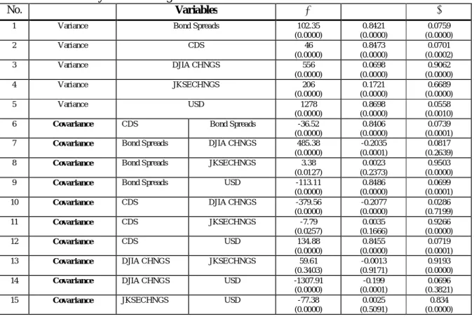
Table 3 Result of Diagonal VECH GARCH Model 58
Table 4 Variance and Covariance Matrix 59
Table 5 Dickey- Fuller Test Result 62
Table 6 Pair wise Granger Causality Tests 63
Table 7 Block Exogeneity Wald Test Result 65
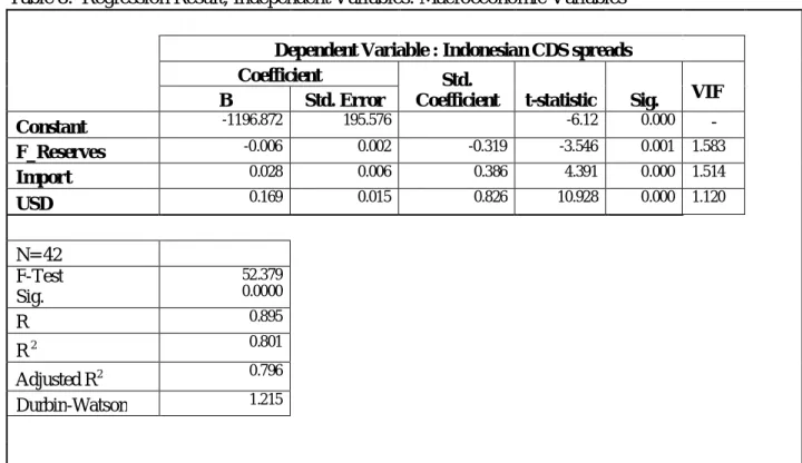
Table 8 Regression Result, Independent Variables: Macroeconomic Variables
66
Table 9 Regression Result, Independent Variables: Macroeconomic Variables and Global Market Sentiment
68
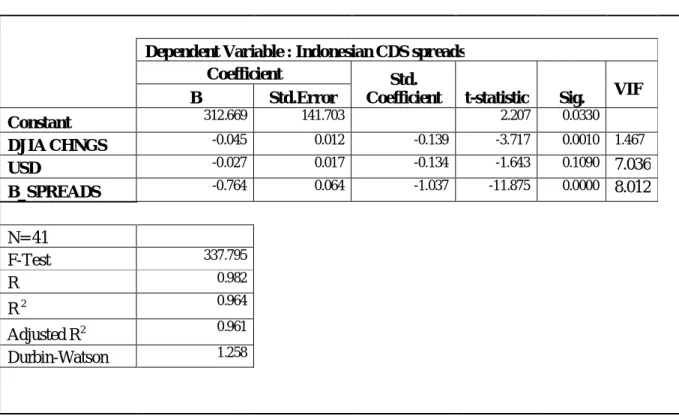
Table 10 Regression Result by Including Bond Spreads as Independent Variable
1
CHAPTER I INTRODUCTION
1.1.Background
Rational investors in all over the world want to maximize their investment return. However, there is constrain limit this objective. The constraint is the risk. High return usually obtained by investing in high risk. On the other hand, low risk naturally generates low return. In this trade- off between risk and return investors will invest their money in such an investment instrument as long as the return excesses its risk.
Market risk and credit risk are the risk included in sovereign bond investment. The example of market risk is the interest rate risk. It is the risk that the interest rate will become higher or lower in the future. If the bond pay a fixed rate interest rate coupon, an increase in current interest rate will make the price of bond decrease and vice versa. On the other hand, credit risk related to risk that a bond issuer cannot pay its obligation at the scheduled time.
Regarding to investing in sovereign bond, different bond issuer carry its own specific risk. In addition to market risk, the specific risk creates different interest coupon set for different bonds.
Trade off between risk and return on investment creates a relation between bond risk and yield asked by investors. Higher risk carried by the bond issued consequently will make the return asked by investors be high. Additional risk needs to be compensated with additional return. From bond issuer point of view, this situation make it has to decrease the price of its bond when the risk is higher. Normally this means that it has to increase interest rate of its coupon.
2
Unites States Treasury Bond is a sovereign bond commonly used as a benchmark for valuing other sovereign bond. Because of its highest creditworthiness, it is assumed that federal government of United States will never go default. Since US Treasury Bond is assumed to be risk free, other bonds are compared to it to measure the risk default.
Bond issuers always want to reduce its cost of borrowing consequently they need to decrease the risk associated by investors to their bonds. While market risk almost always incurred in every bond, credit risk can be assumed to be specific to a bond issuer. Hence, the bond issuer needs to manage its credit risk very carefully.
If government cannot manage the credit or default risk carefully, it will face the higher cost of borrowing as its consequence. Whenever it wants to issue a new bond for financing its budget deficit or refinancing its old bond, the price of its bond will be cheaper than the price in managed default risk. The snow ball effect happens when the government is forced to always issue a new bond due to its unavoidable need. Higher cost of borrowing due to higher interest rate will make its default risk worsened. The cycle will continue whenever it issues a new bond. The end of the game is when the government cannot pay its obligation. This means that default risk is not a mere potential risk again, but it has been transformed to be a real event.
After got hit by Asian crisis in 1997/1998, Indonesia has tried to change its budget deficit financing strategy from foreign debt to domestic debt. Indonesia not only shifted its strategy from foreign debt to domestic debt, but also shifted it from multilateral/bilateral financing to market
3
financing. This strategy is done through bond issuance both in the domestic market and in the global market.
Accumulation of bond issuance from year to year created many questions about country‘s ability to manage its debt, especially its ability to pay coupon and bond principal. The ability to pay coupon and bond principal is reflected by default risk of the bond issuer. Higher default risk of bond issued naturally will be compensated by higher bond yield asked by investors. Default risk then becomes a concern not only for investors/creditors but also for government as bond issuer.
One of accepted instrument to measure default risk of a bond issuer is a derivative instrument which is called Credit Default Swap (CDS). CDS spreads or sometimes it is called CDS premium shows market valuation and perception about probability of one bond issuer to be in a default situation. Function almost similar as insurance premium, CDS spreads shows money to be paid for covering a credit default event. The higher a probability of one bond issuer to default, the higher CDS spreads of that issuer.
During the financial crisis in year 2008, Indonesian government bond CDS spreads jumped significantly from its level in year 2007. Additionally, the increase of CDS spreads was accompanied by difficulty in issuing new bond due to very high yield demanded by investors. At the same time, there was a shock in the stock market all over the world leaded by shock in Wall Street.
4
On the other hand, Indonesian macro economy even though got impact from financial crisis seems to be resilient. This was proven by relatively only little decrease in economic growth. Hence, the crisis and its impact to Indonesian ability to issue a new bond created questions about the relationship between Indonesia CDS spreads, macroeconomic factors, and sentiment in the stock market.
Figure.1. Indonesian Credit Default Swap Spreads: January 2007- July 2010 (basis points)
Source: Bloomberg
1.2 Research Question
Previous studies have confirmed that macroeconomic variables are significant in explaining emerging market bond spreads empirically (Cantor & Packer, 1996; Amato & Luisi, 1996; Min, 1998; Eichengreen & Mody, 1998).
0.00 100.00 200.00 300.00 400.00 500.00 600.00 700.00 800.00 900.00
5
Using the same logical reason, this research investigates the role of macroeconomic variables and additional variables to explain variability of Indonesian CDS spreads. This research is trying to find an explanation of fluctuation in Indonesian CDS spreads during January 2007 to July 2010. Market sentiments reflected by changes in the stock market index is chosen as additional explanatory variables.
1.3 Research Structure
This research offers a statistical test to find some better additional variables to be included in further analysis. Relationship amongst variables using available daily data is investigated using Generalized Auto Regressive Conditional Heteroscedastic (GARCH) model.
Market sentiments are differentiated between domestic market sentiment and global market sentiment. Granger causality tests are constructed to investigate the role of both sentiments in predicting Indonesian CDS spreads.
Several macro economic variables are investigated using regression analysis to find their explanatory power of Indonesian CDS spreads. Finally, macroeconomic variables and market sentiment are combined as independent variables in regression analysis. This method is taken to find a model which describes the role of macroeconomic variables and market sentiment in explaining fluctuation of Indonesian CDS spreads during the sample period. While daily data is used in variable selection using GARCH model and Granger causality test, monthly data is used in regression analysis.
6
Different from most of previous studies which used panel data in their analysis this research uses time series data. Time series data is chosen to find a better explanation of specific relationship characteristic between country fundamentals, market sentiment and credit default risk.
Even though several macroeconomic variables, such as Gross Domestic Product (GDP), GDP growth, term of trade, debt service ratio, have been found to be significant in explaining CDS spreads or bond spreads, they cannot be used in this research due to data availability.
Gross Domestic Product (GDP), GDP growth, and several variables which use GDP as ratios can only be acquired at most in quarterly data or annually data. They are little of use in explaining CDS spreads fluctuation in a short term or medium term.
It is difficult to convince that variables which changes quarterly or annually can be used to explain daily variability of CDS spreads. Instead, monthly data is chosen to find the closest explanation of Indonesia CDS spreads fluctuation during January 2007 to July 2010.
Relationship amongst five variables, Indonesian CDS spreads, US Dollar rate, Bond Spreads, Changes in Dow Jones Industrial Average index, and Changes in Jakarta Stock Exchange index, is investigated using symmetric diagonal VECH GARCH model. Daily data of those variables are used in this analysis. Moreover, the result of this model is also used to select one of two macroeconomic variables, Bond spreads and US Dollar rate. It is revealed from covariance parameters obtained from the model that US dollar rate is a better variable than Bond spreads to explain Indonesian CDS spreads.
7
To investigate the role of global and domestic market sentiment to Indonesian CDS spreads Granger causality test is conducted. The global market sentiment is reflected by changes in Dow Jones Industrial Average index while the domestic market sentiment is reflected by changes in Jakarta Stock Exchange index. The Granger causality test result suggests that, global market sentiment is a better variable rather than the domestic market sentiment to explain Indonesian CDS spreads.
Macroeconomic variables regression analysis result shows that two variables, export and inflation, are not significant in explaining Indonesian CDS spreads. Three macroeconomic variables which are Foreign Reserves, US Dollar rate, and Import are significant.
Next, including global market sentiment in regression analysis provides two variables in the final model. They are US Dollar rate and Changes in Dow Jones Industrial Average Index.
Additionally, this research also investigates additional variable, Bond spreads, to explain Indonesian CDS spreads fluctuation. At the same time, this step is taken to confirm variable selection method suggested by GARCH model conducted before. The result shows that including bond spreads variable disturbs the role of previous two variables due to multicollinearity problem. As the result, this additional variable is not included in the final model. The final model consists of two variables which are US Dollar rate and Changes in Dow Jones Industrial Average Index.
Remainder of this research is organized as follows: Chapter II provides some theories and literature review of empirical studies regarding emerging bond market and default risk. Chapter
8
III presents consideration in selecting independent variables and hypothesis. Chapter IV explains data and methodology used in this research. Chapter V presents a description of Indonesian Government Bond. Chapter VI presents empirical result of tests conducted and managerial insight. Chapter VII presents a summary and conclusion.
9
CHAPTER II LITERATURE REVIEW
2.1 Default Risk Indicators
History of the world, especially started in 1970s recorded some countries which have problems in paying their debts. Argentina, Brazil, Mexico is an example of countries which had to struggle to survive in managing their debts (Mauro, Sussman & Yafeh, 2006). Recently, Greece has almost the same problem in paying its debt. This situation creates a potential risk that it may happen to other countries, as well.
In order to give market players information about probability of default of one entity, several default indicators are created and computed. For sovereign entity default risk probability, examples of the indicators are credit rating, debt to GDP ratio, bond yield spreads, and CDS spreads.
2.1.1 Credit Rating
Credit rating or bond rating is a current opinion about credit worthiness and quality of a bond issuer to pay its obligation (Jones, 2010b, p.35). Bond rating is issued by rating agencies and is available for investors to analyze and measure default risk of a bond issuer. By using the credit rating, investors can calculate the expected return to compensate the risk incurred in the bond. Moreover, investors can compare the price of bond offered by different issuer by comparing its credit rating.
10
There are many rating agencies in financial market. Each rating agency uses its own rating to presents creditworthiness of a bond issuer. For example, Standard & Poor’s and Moody’s use letters represents a creditworthiness of a bond issuer. The highest rating in Standard & Poor’s system is AAA which represents an extremely strong capacity to pay interest and repay principal of its bonds.
It is important to understand that credit rating is an opinion about prediction of creditworthiness of a bond issuer. Likelihood to be default is used as a single indicator of the creditworthiness. Rating agency such as Standard & Poor’s put emphasizes on order and rank of creditworthiness of bond issuers (Standard & Poor’s, 2009). Then credit rating should be seen as a relative position in the creditworthiness of one bond issuer compares to others.
Additionally, the rating agencies divide its rating system into two broad criteria which are investment grade and speculative grade. The investment grade is credit rating from AAA through BBB in Standard & Poor’s system. They represent a high quality of a bond issuer. Consequently, because of trade off between return and risk, bonds issued by this bond issuer offer a lower return. The other criterion is speculative grade. It is the grade of ratings of bond issuers from BB, B, and CCC, to CC. Because their default risk is higher the bonds they issue have to be offered in a higher return.
Even though credit ratings are accepted by most investors, they have some shortcomings. There is a probability that rating agencies may give different opinion about credit worthiness of one
11
bond issuer. It is normal that one rating agency may give a higher rating to one bond issuer compare to that given by another agency (Jones, 2010b).
Another shortcoming of the rating system developed by rating agencies is that it may be too broad. It cannot be used to explain why, other things being equal, two governments in the same category of rating may have different price of their bonds. Moreover, rating agencies recently have reliability problems. Their methodology to measure default risk is questioned by many financial market players (Partnoy, 2009 p.175-191). Enron case in year 2001 and recent subprime mortgage crisis in year 2008 were examples when rating system did not work well to at least give a signal about potential problem in both cases.
The other problem in credit rating is their ability to follow rapid market dynamics. It is very common that they are left behind in predicting creditworthiness of one bond issuer compare to investor reaction in the stock market or bond market (Jones, 2010b).
2.1.2 Debt to Gross Domestic Product (GDP) Ratio
It is natural to associate a default probability of one country with its economic capacity, which is commonly measured by its Gross Domestic Product (GDP) (Jones, 2010a). While debt to asset ratio measures leverage of corporate, debt to GDP ratio can be assumed measures leverage ratio of one country. The probability of default is assumed to be high when the amount of debt high. Hence, the ratio of debt to GDP intuitively can be used to measure the ability of one country to pay its debt obligations.
12
By using this logic, the lower ratio of debt to GDP means the higher creditworthiness of a country while the higher ratio means a vice versa situation. The higher ratio means the country becomes more vulnerable to be in a default situation. This ratio is reasonable. If accumulative debt is excessively high compare to total country’s production, and then the country ability to repayment its debt becomes weak. Total production has to be used to other needs not only repaying debts. Moreover, gross domestic product reflects potential tax revenue can be collected by government. If the ratio of debt and gross domestic product is 5 %, then simply by increasing the tax rate by 5 % government can wipe out the debt accumulated for that year (Jones, 2010a).
While some countries still survive and can manage their debt well even though their current debt to GDP ratio relatively high, some other countries does not. Japan, United States and other developed countries are countries which have a ratio of debt to its GDP more than 100 %, but they seem do not have a problem in managing their debt. It can be seen from high credit rating of these countries. Jones (2010a) emphasizes the argument that there is not a magic level of debt to GDP ratio can be used to predict debt crisis. Economic size and growth prospect of the country will be the most important consideration to measure government ability to collect taxes and minimize spending (Jones, 2010a p.395).
Another shortcoming of using debt to GDP ratio for predicting default risk is a fact that GDP figure at most can be gained by quarterly data (Beck, 2001). Measuring the figure in monthly or weekly data is not easy to do. On the other hand, financial situation can change dramatically within a short period less than one month or even one week in a financial crisis situation.
13 2.1.3 Bond Yield Spreads
Bond yield spreads or bond spreads is a measurement of credit risk incurred in one bond compared to risk free instrument such as Treasury bond. While it is assumed that Treasury bond is a risk free rate instruments, the difference between yields of Treasury bond and yields asked by investors to particular sovereign bond of the same maturity reflecting credit risk perceived by investors and additional return asked because of holding riskier instruments.
The nature of logic behind bond yield spreads measurement is very convincing. It assumes that difference of those yields reflects the default risk incurred by particular bond issuer. However, previous study has revealed that what makes those yields different is not mere default risk (Küçük, 2010). There are certain factors influence yields asked by investors. Some of them are liquidity and tax factors.
Illiquid instruments such as some emerging market bonds got penalty by investors by asking a higher yield. Investors face the risk that they will not easy to buy or sell the bond because the instruments are illiquid. In this case, investors need to compensate this risk by asking higher return. The risk actually has nothing to do with probability of country default but mere illiquid problem.
Changes of tax policy in United States can ignite new calculation of Treasury bond yield. There will be an increase or decrease in yield spreads which is not caused by changes in default probability. Hence, bond yield spreads may not reflect a pure default risk as it is aimed.
14
Additionally, it is very difficult to compare two identical bonds in regard of time to maturity and schedule of coupon payment. At most, the bond spreads reflects the closest comparison only.
2.1.4 Credit Default Swap Spreads
Derivative instrument that relatively newly introduced is Credit Default Swap (CDS). This instrument offers a pure measurement of default probability of a bond issuer. The CDS spreads theoretically only deal with default risk (Beck, 2001; Benkert, 2004). Generally credit swap is a financial instrument where its value depends on credit quality of debt issuer, private or government (Chisholm, 2010 p.75).
Duffie and Singleton (2003) define credit swap as a form of derivative security that can be viewed as default insurance on loans or bonds. Credit swap offers protection of a credit event by giving the buyer a given contingent amount of at the time of a given credit event. The contingent amount most often is specified to be the difference between the face value of a bond and its market value, paid at the time of the credit event. As a return for the protection, the buyer of protection pays a premium, in the form of an annuity, until the time of the credit event or until the maturity date of the credit swap, whichever is first (Duffie & Singleton, 2003 p.173)
Credit swap can be seen as default insurance where swap buyer protects itself from losses caused by default event of bond it bought. Since each bond carry a default risk in it, one can buy a protection scheme for every bond traded in the market to ensure that cash flow expected from the money invested in that bond can be realized.
15
As well as bond yield spreads, the CDS spreads data which can be quoted daily reflects daily valuation and measurement of investors about default probability of a bond issuer. Especially for emerging bond market, CDS market is more liquid than the bond market. It has flexibility in maturity which is sometimes not available in underlying bond (Chisholm, 2003 p.77).
Ericsson, Jacob & Oviedo (2004) also mentions the advantages of using credit default swaps data rather than using bond yield spreads data. Default swap spreads do not need to be adjusted to reflect default risk because it is already a default risk premium. Moreover, they argue that default swap spreads offer a more accurate and quicker response to changes in credit risk than bond yield spreads.
2.2 Credit Default Swap Market and Mechanism
Credit Default Swap is traded in Over The counter (OTC) market. This means that transaction and contract of credit default swap is not conducted in an exchange market. Instead, the transaction depends on agreement between the seller and buyer. Because of potential dispute between the seller and buyer in defining a credit event and the other thing stipulated in credit default swap contract, there is an organization which minimizes the probability of dispute amongst parties. Terms of credit default swaps is standardized by The International Swaps and Derivatives Association (ISDA). The association also collects and files any information related to credit risk such as bankruptcy, cross default, rating downgrade, failure to pay, repudiation, and restructuring (Duffie & Singleton, 2003 p.175)
16
When an entity wants to buy a credit default swap contract for one bond issuer, it can go to a credit default swap seller and negotiate terms of contract based on standard stated by ISDA. In this case, CDS contract is different from an insurance contract. The buyer does not necessary already have a reference asset to be protected for. Instead, the buyer can buy the reference asset at the time of a credit event or sell the CDS contract to another buyer anytime it wants to.
The premium which is paid annually is called spread and it is said in basis points. The spreads times its protected amount will show the annual payment should be paid by the buyer of credit defaults swap to the seller.
CDS buyer who does not have the underlying bonds in its hand can gain profit in two ways. If the CDS buyer sees creditworthiness of its reference entity decreases, it can sell its CDS contract to a new buyer who wants to protect its position. The old buyer will get higher premium from the new buyer. The profit is margin between new premium revenue from new buyer and old premium should be paid by old buyer to CDS seller. Alternatively, the CDS buyer can hold the contract until such a credit event occurs. It can buy a cheaper reference bond in the bond market, delivered it to CDS contract seller and get a par value of the bond (Chisholm, 2003 p.77).
2.3 Determinants of Default Risk and CDS spreads
Chisholm (2003) defines credit default swap as a derivative instrument which its value has a very close relationship with reference entity creditworthiness. Hence, it is naturally that measuring the spreads of CDS also means measuring creditworthiness of an entity.
17
Creditworthiness or credit quality of government cannot be separated from economic performance of one country. Many scholars have investigated macroeconomic factors that offer an explanation of credit quality as measured by default risk indicators.
Duffie and Singleton (2003 p.149) lists some of macroeconomic factors including its sign relationship that are highly possible to influence a country’s ability to pay its debt obligation. They are current account to Gross Domestic Product (+), terms of trade (+), reserves to imports (+), external debt (-), income variability (-), export variability (-), and inflation (-).
Additionally other variables to explain creditworthiness of one country are introduced by many studies. Cosset & Roy (1991) try to replicate Euro Money and Institutional Investment country risk rating by using economic and political variables. They find that countries which have high quality country risk rating are less indebted country compare to low rating countries. Important finding from their study is the ability to replicate country risk rating calculation in a significant degree by using only available economic statistics.
Alesina et al. (1992) investigates the presence of default risk for Organizations for Economic Co-operation and Development (OECD) countries. By comparing interest rate on government and corporate financial instruments, they find a strong relationship between the amount of government debt, and the difference of government and corporate rate of return. In addition, they find the existence of investor perception about default risk of OECD countries. Even though the portion of default risk perception is very small, it shows that investors distinguish every financial instrument by incorporating a default risk consideration in determining rates of return.
18
Cantor & Packer (1996) argue that Moody and Standard & Poor’s rating announcements can be explained by a small number of well-defined criteria. Using several variables such as Per capita income, GDP growth, Inflation, Fiscal Balance, External Balance, External Debt, Spreads, Indicator for economic development, and Indicator for default history, they find that market, gauged by sovereign debt yields, broadly shares the same sovereign credit risk made by the true rating agencies. They argue that credit rating appears to have some independent influence on yield over and above their correlation with other publicly available information. Moreover, they investigate the impact of rating announcement to market pricing. They can show that rating announcement has immediate effect on market pricing for non-investment grade issues.
Packer & Suthipongchai (2003) report that within the same rating in high rating levels, sovereign CDS spreads is lower than corporate CDS spreads. However, they cannot conclude that the reason for this phenomenon is caused by whether liquidity factors or limited sample. On the other hand, the reserve phenomenon occur for low rated sovereigns and corporate. Spreads for low rated sovereigns is higher than spreads for low rated corporate. Explaining the latter phenomenon, they argue that this occur because investor becomes more pessimists about recovery rate of sovereigns default compare to that of corporate.
Min (1998) in his study tries to get determinants of credit risk. Min divides explanatory variables of emerging bond spread into two categories which are liquidity and solvency, and macroeconomic fundamentals. The first group of variables relates to short term country’s ability to pay its debt obligations while the latter more focus on long term one. Variables included in the first group are the debt-to-GDP ratio, debt-service-ratio, net foreign assets, international
reserves-19
to-GDP ratio. The second group of variables consists of domestic inflation rate and terms of trade. Additionally, Min uses oil price and international interest rate as external shock to formulate its model. It is found that liquidity and solvency variables (debt-to-GDP ratio, international reserves-to-GDP ratio, and debt service ratio and export and import growth rates) are significant in determining yield spread. In addition, inflation rate, net foreign assets, terms of trade and real exchange rate are found to be significant in explaining the spreads. Interesting finding is that external shock variables are not significant to explain the yield spreads in his model.
Beck (2001) argues that emerging market Eurobond spreads after the Asian crisis can be almost completely explained by market expectation about macroeconomic fundamentals and international interest rates. Beck (2001) study shows that external shock in international interest rate is significant in explaining bond spreads. However, different external shock, reflected in the stock market volatility in the developed countries, did not play a significant role after Asian crisis.
Amato & Luisi (2006) investigate the role of macroeconomic variables in estimating the arbitrage-free rate structure models of yield and spreads of United States Treasury and corporate bonds. They find that the measurement of default risk event varies between high and low rate bonds. More importantly, it is suggested that additional compensation for the default event risk is not pro cyclical.
Ludvigson & Ng (2009) study reveals the importance of real and inflation factors in predicting excess returns of US government bonds. This predicting power is beyond the power incurred in yield spreads. This finding implies that without including the macro factors risk premium
20
appears virtually a-cyclical, whereas with the estimated factors risk premium have a marked countercyclical component. It is then consistent with theories that investors must be compensated for risks associated with macroeconomic activity.
Hilscher & Nosbuch (2010) investigate the effect of macroeconomic factors in sovereign risk. Using data of emerging market sovereign credit spreads; they find that terms of trade volatility has a significant effect to the spreads. This finding implies that focusing on terms of trade of country specific commodity price index in analyzing and distinguishing the relation between macroeconomic factors and sovereign risk can be done.
The importance of market sentiment for explaining CDS spreads is investigated by Tang & Yan (2010). They argue that during GDP growth rate credit risk premium in average decreases. The reserve phenomenon occurs when there is a fluctuation in GDP growth and shock in the stock market. They conclude that credit risk premium is determined mostly by market sentiment at the market level. For corporate level, they find that the most powerful factor in explaining the risk premium is implied volatility. Macroeconomic factors are found to be has a direct impact but only for a smaller portion.
Using quintile regression, Pires, Pereira & Martins (2010) argue that what they called traditional variables such as solvency factors, volatility, cannot fully explain the level of CDS spreads. The liquidity cost is also reflected in the spreads. Illiquid instruments will be penalized by higher credit risk spreads compare to the liquid ones. In investigating and measuring transaction cost for
21
CDS, they argued that it must be done by using absolute figure rather than a difference between bids and ask figures.
2.4 CDS Market, Bond Market, and Stock Market Relationship
Study to find a relationship amongst CDS market, bond market and stock market has been conducted by many scholars (Forte & Pena, 2009; Norden & Weber, 2009; Frank & Hesse, 2010, and Ismailescu, 2010).
The impact of common market sentiment to both domestic and foreign debt was investigated by Hanson in year 2007. Hanson (2007) argues that the composition of debt whether foreign or domestic should not be overstated. Excessive debt and negative shocks can contribute to a “sudden stop” in the demand for both government domestic debt and government foreign debt. The current attractiveness and low cost of domestic debt may reflect the international environment not fundamental changes. Panizza (2008) has also mentioned about the danger of strict differentiation between domestic and foreign debt.
Norden & Weber (2009), using data span from year 2000-2002 of corporate bond, stock and its credit default swap, investigate the inter temporal co-movement of those variables. They use Vector Autoregressive (VAR) model to study the lead-lag relationship and causality. The Granger causality test is conducted by using different terms of data which are monthly, weekly, and daily data. They find that changes in CDS spreads Granger causes bond spreads changes for more firms in United States and Europe rather than vice versa. They also argue that credit default
22
swap market is more sensitive to stock market than the bond market. Additionally, they find that larger bond issues and lower credit quality increase the co-movement amongst those markets.
Correlation between credit rating and credit default swap may seem a perfect correlation. Whenever credit rating deteriorates or increases, logically the possibility to default will increase or decrease as well. Consequently, credit default swap also will increase or decrease. However, credit risk changes may be anticipated differently by investors in credit default swap market and rating agencies. Credit rating announcement may take more time than changes in CDS spreads. Investor may have already incorporated information contained in credit rating announcement far before it is announced by rating agencies. On the other hand, rating announcement may enforce investors to re-calculate their perception about credit risk of particular issuer. The impact of credit rating announcement on country’s credit risk then becomes an interesting subject to be analyzed (Cantor & Packer, 1996; Ismailescu, 2010).
Ismailescu (2010) finds that CDS spreads anticipate positive events (higher credit rating) announcement more than it anticipates negative events. On the other hand, CDS spreads are better in forecasting a probability of credit rating downgrade. Ismailescu (2010) also argues that financial factors were able to explain changes in CDS spreads better than macroeconomic factors or political factors.
While most of the studies confirmed the existence of parallel relationship between credit risk premium and bond yield spreads, Adler & Song (2010) reject this direct relationship. They find that negative spreads in bond yield sometimes can result in positive credit risk premium and
23
vice versa. They argue that the phenomenon is caused by non-par price. By constructing this non- par price through implied bond yield spreads, they can reestablish parity relationship between credit risk premium and bond yield spreads for the most part of their sample. However, unparalleled relationship still can still be found in some cases (Adler & Song 2010).
24 CHAPTER III
VARIABLE CONSIDERATION
This research tries to find an explanation of fluctuation in Indonesian CDS spreads during time January 2007 to July 2010. Since it relates to only one specific country, variables will be used in the analysis should be determined carefully based on the appropriateness of measurement and the availability of data.
Previous studies have been exploited broad types of variables to explain credit risk represented previously by bond spreads and recently by CDS spreads. Table 1 summarizes variables used in several previous studies. In general, variables used in previous research can be divided into two broad types. They are macroeconomic variables or fundamentals, and additional variables. Using the same logic of previous studies, this research uses macroeconomic variables to explain a country’s credit risk, in this case is Indonesian CDS spreads. Dependent variable then is Indonesian CDS spreads. Independent variables will be divided into two parts. The first part is macroeconomic variables, and the second part is market sentiment. Since sample period used in this research is argued had been influenced by fluctuation in the stock market, market sentiment is chosen as additional variable. Market sentiment measurement is represented by using changes in the stock market index.
3.1 Data Level
Level of data to be used to investigate the relationship amongst CDS spreads, macroeconomic variables and market sentiment may vary from daily, weekly, monthly, to annually. The choice
25
depends on the purpose and the reason of the research to be conducted. Each choice, however, has its own advantages and shortcomings (Beck, 2001).
Table. 1. Independent Variables Used in Previous Studies
Independent Variables Eichengreen & Mody (1998) Min (1998) Goldman Sachs (2000) Beck (2001) Abid & Naifar (2010) Ismailescu (2010) Quarterly/
Annually Debt/GNP External Debt/GDP External debt/GDP
External Debt/GDP Growth rate of GDP International Reserves/GDP Current
Account/GDP Budget Balance
Government Deficit
Growth rate of GDP Real GDP Growth
Macroeconomics
/ Fundamentals Monthly
Debt
Service/Exports Debt Service/Exports
Forecast for Current Acoount Deficit External Debt/Export Growth rate of Export Gowth rate of Imports Terms of Trade(Export/Import)
Net Foreign Assets Foreign Reserves
Inflation
Forecast for
Inflation Inflation Rate
Real Exchange Rate
Real exchange rate
Misalignment US Dollar Rate
Forecast for Real GDP Growth Bond Spreads Additional Credit Rating Residual Opennes of the economy Rating Amortization/Reserv es International Interest Rate International Interest
Rate Long run LIBOR LIBOR
Free Risk Interest Rate
Domestic Market sentiment
Real Oil Price
Time to Maturity Credit Rating Events Slope of the yield curve (long-short Interest rate) Composite index of Polical risk Volatility index Volatilities of Equities
26
Most of previous studies used panel data, consist of several countries data, to get general explanation of sovereign credit risk (Eichengreen & Mody, 1998; Min, 1998; Beck, 2001; Abid & Naifar, 2010; Ismailescu, 2010). Hence, annually or quarterly data could be used for their researches. On the other hand, this research tries to explain specifically credit risk of one country only, Indonesia. As a consequence, another approach is needed to get a proper result by considering data availability and the aim of this research.
Using daily data for investigating the relationship between credit default swap market and stock market will not have a problem in data availability. Both markets record any information needed daily. However, daily data should be used carefully. News and rumors sometimes affect those markets more than fundamental issues (Beck,2001).
Data availability will be another concerns should be taken care in doing this investigation. Fundamentals macroeconomic variable such as Gross Domestic Product (GDP) growth is released at most quarterly. Inflation rate, export, import, inflation and the level of country foreign reserves can be accessed at most in monthly data. Hence, to obtain the closest relationship between CDS spreads and macroeconomic variables it is argued that using monthly data is the most appropriate method.
Using monthly data in investigating the relationship between CDS spreads and macroeconomic variables offers the closest approach to reveal investors’ decision and calculation based on the true publicly available data. Moreover, averaging the daily data into monthly data will minimize
27
the effect of unrelated rumors to changes in credit default swap market or stock market (Beck, 2001).
There is a consequence of using monthly data strictly. Some variables which theoretically important in estimating credit worthiness of one country and its credit default swap spread, such as debt to GDP ratio or credit rating, may not be able to be included in the analysis. Some scholars tried to bridge the gap between quarterly or annually data and monthly data by transforming it using interpolation technique or using forecast of the data (Beck, 2001). However, it is argued that interpolated data is “interpolated data” which means that they do not reflect the actual data of variable itself. Some subjective judgments and assumptions are extensively used to get the data.
Since the research is implicitly trying to reveal investor behavior and perception about default risk, interpolated data will not be used. Hence, some variables suggested by theories and other studies are excluded from the research not because they are not important but because of the research purpose and data limitation.
3.2 Macroeconomic Variables
Macroeconomic variables used by previous studies to explain credit risk of one country can be presented in various forms. Each scholar as it is presented in Table 1 emphasizes the importance of selected variables to represent a country’s ability in honoring its obligation. Using the same logic used in Beck (2001), this research will use monthly data in regression analysis. Since this
28
research will use monthly data in regression analysis, the available macroeconomic variables are Bond Spreads, US Dollar Rate, Export, Import, Foreign Reserves, and Inflation rate.
3.2.1 Bond Spreads
Bond yield spread or bond spreads has been widely used as one of credit risk indicator of a bond issuer (Eichengreen & Mody, 1998; Beck, 2001). The explanatory power of bond spreads to represent a country’s economic performance is based on its direct comparability with others country economic performance.
Benchmark for bond spreads is the yield of US Treasury bond with the same maturity. Wider spreads reflects higher credit risk of a bond issuer. In a situation where another country issues the same maturity bond but with less wide bond spreads, this implies that its economy is worse than another country’s economy..
Since Bond spreads basically measure credit risk of bond issuer as well as CDS spreads, their relationship is expected to be in positive one. Wider bond spreads intuitively should be accompanied by higher CDS spreads and vice versa.
3.2.2 US Dollar Rate
US Dollar nowadays stills the most important currency in the world proved by the fact that many economic activities are measured by US Dollar equivalent. Export, import, foreign reserves, and many others activities are examples of economic activities measured by US Dollar to represent
29
the country’s economy. Using the US Dollar currency as standard measurement offers an easy comparison of countries economy to others.
Foreign exchange rate shows the power of one country economy compare to another one. Weak domestic currency reflects a weak economy relatively and vice versa. Moreover, exchange rate also reflects how well the economy is managed by the government (Jones, 2010a).
Changes in the exchange rate will give impact to many economic activities in one country. International trade will get the first impact. Revenue and cost of doing international trade depends heavily to fluctuation of exchange rate (Jones, 2010a). In regard to government foreign debt management, the fluctuation of exchange rate will make the nominal amount of debt and its following obligations measured in domestic currency also will fluctuate. Since most part of government revenue is generated by domestic tax revenue, the domestic currency depreciation will hamper the country’s ability to pay its debt obligations. Consequently, when domestic currency is devaluated severely, the probability of credit default will increase. Since higher US Dollar exchange rate gives a positive contribution to higher default risk, expected sign of this variable in regression analysis is positive.
3.2.3 Export
Export activities measure economic activities of one country and the role of it to the world economy. In globalization and trade openness era, a country which is able to increase its export value normally will get higher benefit for its own economy (Jones, 2010a). Moreover, export value also reflects the role of one country’s economy in the world economy.
30
One of source of foreign reserves for most of countries in the world come from foreign currency revenue generated from export activities. Regarding to country ability to pay its foreign debt, the higher the export value will offer the higher ability to pay the country’s financial obligation. Increasing the value of export generates more money for the economy. Hence, it is hoped that there will be a negative relationship between value of export and default risk of one country.
3.2.4 Import
Import activities create cash flow from the host country to others countries. When import mainly consists of consumptive goods and services, the value of import reflects the inability of one country to produce its needs for economic activities. On the other hand, when import consists of productive goods and services which were used to produce new products by including value added to be exported to other countries, then import activity is a necessary condition to improve country economy (Jones, 2010a).
However, from cash flow point of view, import activity is cash out flow activity. This means the activity is part of activities that need to be funded by country’s economy. The higher the cash needed to fund import activity, the less cash remain to fund others activities. Hence, the relationship between import value and country ability to pay its debt obligation is expected to be in a positive relationship.
3.2.5 Foreign Reserves
Foreign reserves are the measurement of how much deposits and bond foreign currency owned by government or monetary authorities. The level of foreign reserves reflects country ability to
31
fund its obligation in paying international economic activities. The activities include importing and paying coupon and principal of government bond. Higher foreign reserves level shows higher ability to pay international financial obligations (Jones, 2010a). In regard to default risk of government bond, the higher level of foreign reserves means the lower level of default risk. Consequently, CDS spreads as a measure of default risk will be lower.
Level of foreign reserves changes depends on foreign currency cash inflow and outflow. Source of foreign currency cash inflow not only come from export activities but also from several financial transactions. The examples of the transactions are remittance from foreign country, and foreign currency denominated government debt issuance. Cash outflow of foreign reserves mainly caused by import transaction and international financial obligations.
3.2.6 Inflation rate
Inflation rate is one of indicators which can be used to measure how well economy of a country is managed (Jones, 2010a p.202). High inflation tends to show a bad sign of economic management. Managed inflation accompanied by economic growth is a required condition for sustainable economic growth. Related to investing in government debt instruments, high inflation means a decreasing in the real income gained by investors. Since there is not investor who wants to see its future income decreases, it will naturally react negatively to information about high inflation.
The relation of inflation and bankruptcy rates was investigated by Wadhwani (1986). The study confirmed that inflation increase bankruptcy rate and default premium for private companies.
32
Borrowing the same logic to be used in sovereign bond issuer case, a positive relationship between the inflation rate and CDS spreads can be expected to occur in a regression analysis.
3.3 Market Sentiment, Global or Domestic?
Market sentiment can take the form of the domestic market sentiment or the global market sentiment. Domestic market sentiment represents investors sentiment whether positive or negative to make investment in the domestic market by buying local financial instrument. Related to Indonesian CDS spreads, this sentiment is argued can be used to measure the direct impact of investors desire to invest in Indonesian financial instrument without differentiating between corporate or government instruments. Positive market sentiment is represented by positive changes (current index is higher than previous index) in Jakarta Stock Exchange index, while negative market sentiment is represented by negative changes.
On the other hand, global market sentiment is measured by using developed stock market index changes. Since United States is the most leading financial market in the world, the index changes in this country are used as a proxy of the global market sentiment. The market sentiment represents global investors desire to invest their money in riskier financial instrument around the world. Hence, positive market sentiment will be represented by positive changes in US market index and vice versa. Dow Jones Industrial Average Index is chosen to reflect global market sentiment.
Dow Jones Industrial Average index is perhaps the most known and the most quoted index in the world. The Dow Jones name comes from The Dow Jones & Company the publisher of The Wall
33
Street Journal. The index is computed from 30 stocks selected by the company. The index due to its historical background carries a unique index compares to others index which come later, such as Standard & Poor’s 500. The Dow Jones index uses price-weighted index rather than market value-weighted index. Consequently, the index gives a higher weight for higher-priced stocks rather than the lower priced stocks. It is implied that since 30 stocks were chosen selectively from the most leading stock in each industry they carry the same market value. One important thing should be mentioned about the index is its divisor. Because stocks that are used to compute the index has been changed several times, the Company has to make sure that any changes except the changing of stock price including in the index, will not change the index (Jones, 2010b p.92).
The index which measures stock price changes in Jakarta Stock Exchange is well known as Jakarta Composite Index (JCI). Different from the Dow Jones Industrial Average index, the Jakarta Composite Index does not use price weighted average index, but market value weighted average index. The index uses all companies stock market value listed in the market. Market value is calculated by timing closing price times and its nominal amount of stocks listed. The base value for index calculation uses 10 August 1982 as the base market value.. As well as the Dow Jones Industrial Average index, the company which responsible for index calculation adjusts any changes in the stock market that do not make the price of index changes such as a stock split and introduction of a new stock.
3.4 Variable Selection Method
There are two variables can be used to reflect a country’s fundamental by using daily data. They are Bond Spreads and US Dollar Rate. Daily data for both variables can be accessed from market.
34
To explain Indonesian CDS spreads the goodness of using both variables or using one of them should be investigated first.
The same situation occurs for market sentiment variables. Global and domestic market sentiment relationship may need to be investigated first before put them in regression analysis. Based on the phenomenon of Indonesian CDS Spreads and stock market index in United States and Indonesia it is argued that market sentiment has a relationship with the spreads. However, which market sentiment can be used to explain better variability of Indonesian CDS spreads is not easy to determine. Even though both market sentiments seem to have nothing to do with default risk measurement, they may offer additional information for explaining variability of Indonesian CDS spreads.
Ismailescu (2010) uses domestic market sentiment, measured by domestic stock exchange index, as additional variable in the study to reveal determinants of CDS spreads. However, using global market sentiment in this research is compelling due to stock market fluctuation during the sample data. Since there is no base theory to select which market sentiment can be used to explain variability of Indonesian CDS spreads, another approach is needed. The approach should be based on statistical test, the test which does not need a basic theory first. Granger causality test offers such a test of causality based on statistical test.
3.4.1 Symmetric Diagonal VECH Model
GARCH model is one of econometric models recently popular in financial analysis. The model is designed to capture volatility clustering. It is able to capture financial time series characteristic
35
where high volatility followed by high volatility and low volatility followed by low volatility (Seddighi, Lawyer & Katos, 2000; Alexander, 2008;Wang, 2009; Francq & Zakoïan, 2010).
Generalized Auto Regressive Conditional Heteroscedasticity (GARCH) model is a model based on ARCH model. This model is heteroscedastic time varying conditional variance with both auto regression and moving average.
= , ~ (0, ) (1)
= + + ⋯ + + + ⋯ +
= + ∑ + ∑ (2)
Widely adopted GARCH model in the empirical analysis is GARCH (1,1) model where p=1, and q=1. In this simplest case of GARCH model, the conditional variance is:
= + + (3)
In multivariate GARCH model, conditional variance is extended to the conditional variance and conditional covariance. GARCH term usually written in h or H. Hence, multivariate GARCH model known as Vector GARCH can also be written as VECH. The simplest possible multivariate in GARCH model is symmetric diagonal VECH GARCH model. Conditional variance or covariance in this model is written as:
ℎ , = + , + ℎ , (4)
36
In this symmetric Diagonal VECH model, variances can never be negative, and the covariance between two series is the same irrespective of which the two series is taken first (Brooks, 2008 p.434). To explain parameters obtained from the model, plain vanilla GARCH parameters interpretation stated by Alexander (2008 p.137) will be used as guidance.
Alexander (2008) mentions that GARCH error parameter α measure how sensitive the conditional covariance to market shocks. Higher α means that covariance is more sensitive to events in market. How long the impact of market shock to conditional covariance persists will be measured by parameter β; higher β value means that impact of market shock to conditional covariance will persist for a longer time. The sum of α+ β determines the rate of convergence of the conditional volatility to the long term average level. When α+ β is relatively large above 0.99 then the term structure of volatility forecast from the GARCH model is relatively flat. GARCH constant parameter together with sum of α+ β determines the level of the long term average volatility when ω/(1-α- β) is relatively large then the long-term volatility in the market is relatively high (Alexander, 2008 p.137).
Basis of a GARCH model is actually simple linear regression. Hence, it is argued that GARCH model can be used to select a better variable will be used in regression analysis. Its conditional variance and covariance information amongst variables arguably offers a deeper insight about the relationship of those variables rather than offered by conventional Pearson’s Correlation coefficient.
37
Covariance is a measurement of dependency between two assets. Meanwhile, correlation measure the same thing as covariance, but the figure is divided by the product of their standard deviation (Alexander, 2008 pp.94-95). Covariance value can be used to indicate a linear relationship of two variables. Positive value indicates a positive relationship and a negative value indicates the other one. Bigger value indicates stronger linear relationship whether positive or negative (Anderson, Sweeney & Williams, 2011 p. 120).
Additionally, multivariate GARCH imply that the model can capture not only volatility clustering but also clustering in correlation. Since the GARCH model allows covariance and implicitly correlation to be time variant, it is argued that it can capture the financial and macroeconomics time series better than the conventional model. It can give better information about variable relationship in regard to its strength and its sign.
3.4.2 Granger Causality Test
As it defined by Granger (1969), a variable X can be said to be causal of variable Y if past history of X is useful to predict the future state of variable Y over and above knowledge of the past history Y itself. Granger causality then means a precedence where one time series variable changes before changes in another variable (Studenmund, 2011 p.416).
To see if X Granger caused Y, this regression should be run:
38
To find whether X Granger cause Y or not, null hypothesis testing is conducted by stating that the coefficient of X jointly equal zero. F-test will be used to test the null hypothesis. If the null hypothesis can be rejected, conclusion that X Granger causes Y then can be confirmed.
Using the logic in testing of Granger causality, there are three possible results which are unidirectional, bidirectional, and no relationship. Studenmund (2011 p.417) suggests that test the possibility of bidirectional relationship between two variables to conclude a Granger causality relationship is needed.
Before conducting Granger Causality test, all variables included should be in stationary condition. Dickey-Fuller unit root test will be conducted to test stationary condition of each variable. If variables included in the Granger causality test are not stationary in their level form, then the first difference form of variables will be used to conduct the test.
Basically, Granger causality test is a type of Vector Auto Regression (VAR) model. How many lags need to be included in equation should be decided first. There are several ways can be used to decide how many lags will be included in the equation to get a proper result. Brooks (2010, p.293) mentions two broad methods can be used to select proper lag lengths which are cross-equation restrictions and information criteria. Recently the most common approach is using information criterion such as Schwartz Information Criterion or Bayesian Information Criterion, Akaike Information Criterion, and Hannah-Quinn Information Criterion.
39
Of those information criterions, there is not one criterion which is superior to others (Thornton & Batten, 1985). However, Schwartz Information Criterion (SIC), which applies the most severe penalty to additional variables, offers a more consistent model (Brooks, 2009 p.233). Since the SIC offers more consistent model, it is argued that Granger Causality test to do variable selection method using SIC criterion is the most appropriate way.
3.5 Hypothesis
Based on the phenomenon of Indonesian CDS spreads fluctuation from January 2007 to July 2010, theories and literature review presented before, it is hypothesized that Indonesian CDS spreads is a function of macroeconomic variables and market sentiment variables.
Since final investigation of this function will use regression analysis, it is hypothesized that independent variables in this function can explain more than 50 % of variability in Indonesian CDS spreads. Coefficient of determination of regression and adjusted coefficient of determination result will be the measurement of the model obtained.
Null Hypothesis is that the coefficient of determination of regression result is more than 0.5. Alternative Hypothesis is that coefficient of determination of regression result is equal to or less than 0.5. These hypotheses can be written as:
Indonesian CDS spreads = f (macroeconomic variables, market sentiment) H0 = R2 > 0.5
40
CHAPTER IV
DATA AND METHODOLOGY
4.1 Data
Indonesian CDS spreads data is obtained from Bloomberg. It is spreads of a 10 year contract of credit default swap span from January 1st 2007 to July 31st 2010. Monthly data for Indonesian CDS spreads is obtained by conducting arithmetic mean from all available data in respected month.
Bond spread daily data is obtained from the central bank of Indonesia’s website, www.bi.go.id. It is the daily yield spread of government of Indonesia’s bond coded INDO’14. This bond with a nominal amount USD 1 billion will mature in March, 10 2014. Bank of Indonesia presents the spreads in negative value. Higher negative value means wider spreads. As well as Indonesian CDS spreads, monthly data for bond spreads is obtained by averaging all data available in respected month using the arithmetic mean.
Daily data of US Dollar rate for this research is gained from financial data in www. finance.yahoo.com span from January 1st 2007 to July 31st 2010. Arithmetic mean is also conducted to obtain monthly data. The rate is the price of one United States Dollar in Indonesian Rupiahs.
Monthly data for Indonesian export data is gained from Indonesia Statistics Agency’s (Badan
41
Indonesia. The figure is a free on board (FOB) value. The agency presents data of export monthly by its value in US Dollar and the weight of goods exported.
Import data used in this research obtained from Indonesia Statistics Agency’s (Badan Pusat
Statistik) website, www.bps.go.id, which issues it regularly in monthly base. The data consists of data from all area in Indonesia excluding free trade zone area. The value is in Cost Insurance and Freight (CIF) value stated in US Dollar denomination.
Foreign reserves data in Indonesia is issued monthly by Indonesian Central Bank (Bank
Indonesia). Foreign reserves, as reflected by its name, consist of several foreign currencies.
However, the level of foreign reserves is presented in US Dollar equivalent to make it easier to compare with others countries’ economy. Data for this research is obtained from Indonesian central bank website which is www.bi.go.id.
Inflation or deflation rate in Indonesia is measured by measuring increase or decrease in Customer Price Index. Monthly Consumer Price Index (CPI) is obtained by collecting goods and service prices from 66 cities in Indonesia. Generally, goods and services price are calculated using the arithmetic mean. However, there is an exceptional for some seasonal goods and services which are calculated using the geometric mean. Monthly data for the inflation rate is gained from www.bps.go.id.
Additionally, data related to Indonesian debt management is obtained mainly from Debt Management Office, Ministry of Finance Republic of Indonesia and Bank of Indonesia. The data