Choice by iterative search
YusufcanMasatlioglu
Department of Economics, University of Michigan
DaisukeNakajima
Department of Economics, Otaru University of Commerce
When making choices, decision makers often either lack information about al- ternatives or lack the cognitive capacity to analyze every alternative. To capture these situations, we formulate a framework to study behavioral search by utilizing the idea of consideration sets. Consumers engage in a dynamic search process. At each stage, they consider only those options in the current consideration set. We provide behavioral postulates that characterize this model. We illustrate how one can identify both search paths and preferences.
Keywords. Search, satisficing, bounded rationality, consideration set, reference- dependent choice, revealed preference.
JELclassification. D11, D81.
1. Introduction
Classical choice theory assumes that a decision maker (DM) chooses the best option amongallavailable alternatives. This might not be practical, especially in situations where (i) a DM cannot easily view all the alternatives and she must actively seek out alternatives, as when she buys a house or a car (incomplete information), or (ii) there is a menu in front of her, but either the menu is too long or her time is too short (limited cognitive capacity).1 In these situations, the budget set must be explored by the DM. As Herbert Simon pointed out many years ago, exploration of the budget set is one of the most important aspects of real world decision making, but is neglected in the standard theory where the whole budget set is assumed to be evaluated simultaneously.
Yusufcan Masatlioglu:[email protected] Daisuke Nakajima:[email protected]
We would like to thank Tilman Börgers, Kfir Eliaz, Larry Epstein, Fred Feinberg, Michihiro Kandori, Miles Kimball, Kai-Uwe Kühn, Stephan Lauermann, Marco Mariotti, Efe Ok, Emre Özdenören, Doug Smith, Lones Smith, Elena Spatoulas, Ran Spiegler, Neslihan Üler, Gabor Virag, and Frank Yates for their helpful com- ments. Special thanks are due to Steve Salant, Collin Raymond, and Ben Meiselman, who commented on a large portion of the manuscript. We also thank the National Science Foundation for financial support under Grant SES-1024544.
1Although choice overload is usually attributed to the number of options presented to a DM, another source of choice overload could be the number of attributes. Therefore, even with a small number of alter- natives, one may not compare all available alternatives.
Copyright©2013 Yusufcan Masatlioglu and Daisuke Nakajima. Licensed under theCreative Commons Attribution-NonCommercial License 3.0. Available athttp://econtheory.org.
DOI:10.3982/TE1014
This paper proposes a new descriptive model of decision making in which a DM ex- plores her budget set (unlike the standard model) and has a stable preference (as in the standard model). Our procedure is dynamic and incorporates the idea of limited search into a model of decision making. We utilize consideration sets, which have been exten- sively studied in marketing.2 Aconsideration set is the subset of all available options to which the DM pays attention.
While the notion of consideration sets is consistent with standard search theory (Stigler 1961,McCall 1970,Mortensen 1970), there is ample evidence that consumers use heuristic decision rules to determine their consideration sets (Hauser 2010,Gigerenzer and Selten 2001).3 We do not take a stand on which explanations for consideration sets are most plausible. Instead we treat the consideration sets as latent variables and infer both consideration sets and preferences from observed choice behavior.
The novelty of this paper is to model explicitly how the consideration set of a DM evolves during the course of search. The economics literature only recently began to study the effects of limited consideration in market environments (Chioveanu and Zhou forthcoming,Eliaz and Spiegler 2011a,2011b,Goeree 2008,Hendricks et al. 2012, Jeziorski and Segal 2010,Piccione and Spiegler 2012). No one yet has provided a general model of how a DM forms consideration sets over time while choosing among options.
This paper provides such a model by linking the formation of consideration sets to a search process.
Our decision procedure is dynamic because interim decisions about what items to pay attention to affect the evolution of the consideration set. Consider a consumer who is searching for a digital camera. She begins with a tiny amount of knowledge relative to the vast array of products available. Suppose she utilizes an e-commerce site to explore alternatives. First, she looks up a particular camera that she has heard about. Then the website recommends several other cameras. The recommendations influence her choice of what to examine next and when to stop searching. When she stops searching, she chooses the best alternative from the entire consideration set. We call such behav- iorchoice by iterative search(CIS). In this model, the consideration set evolves during the course of search because the items observed during the search (history) trigger ad- ditional search.
There are two plausible interpretations of our model. The first is that the evolution of the consideration set reflects a mental process of the DM. Although there is no explicit search process, the consumer is only able to consider a subset of all available options at any given time. For instance, she may consider only options that are similar to the best item she has already investigated. Under this interpretation, our model becomes a model of an internal process of decision making, even when all options appear to be available.
The second interpretation is that consideration sets are shaped by the environment faced by the DM. For example, a consumer buying items online is often presented with
2SeeHauser and Wernerfelt (1990),Roberts and Lattin (1991), andNedungadi (1990).
3There is also ample experimental evidence that people do not search the way theory predicts (Hey 1982, 1987,Kogut 1990,Moorthy et al. 1997,Zwick et al. 2003,Gabaix et al. 2006,Brown et al. 2011). Instead of optimally searching, subjects use heuristics to decide whether to continue.
options related to what she is examining. These related options, which are provided by the seller, might form the consideration set of the consumer at any given moment. As the consumer clicks through to look at different items, the consideration set evolves.
Although we will discuss our model in terms of search, the reader should keep in mind that the search may be entirely a mental process.
InSection 2we introduce and characterize a general CIS model, where the history and the feasible set affect the consideration set in an arbitrary manner. Because of the generality of the model, inference about consideration sets and preferences is limited.
However, this model is still useful both because it identifies the largest class of choice behaviors that might result fromlimited searchrather than changing preferences and because it acts as a benchmark to compare with models where additional structure is imposed on consideration sets.4
InSection 3, we study a special class of CIS models where each consideration set de- pends only on the best alternative previously observed. This model matches important real world situations, such as Internet shopping websites that recommend alternatives to a product being considered. For example, amazon.com provides information about alternatives in a section called, “What do customers ultimately buy after viewing this item?” The restricted CIS model can be seen as a model of dynamic status quo bias, where the status quo is always the best element in the current consideration set. The current status quo restricts the set of options the DM is willing to consider. The DM will continue to change her status quo until the current status quo is better than all elements in the status quo’s consideration set.
We characterize the model and identify behavioral patterns that are consistent with this consideration set formation process. The restriction improves the predictive power of the CIS model and still allows for choice reversals and cyclical behavior. The restricted CIS model provides richer information about the process that leads up to the final choice and about the DM’s preferences. The restricted CIS model can be used to pin down uniquely the path a DM follows during her search from her choice data.
This analysis assumes that the available data about the DM’s choices are slightly richer than the standard choice data: we observe not only her choice, but also her start- ing point. Thestarting point of a search is the alternative that the DM initially pays attention to. There are many potential reasons for a particular starting point. For exam- ple, a starting point could be (i) the default option, (ii) the last purchase or status quo, (iii) a product advertised to the DM, or (iv) a recommendation from someone in the DM’s social network.5 With the explosion of data mining technologies, observability of such data is more plausible. Nevertheless, it is conceivable that starting points will not be observable in some situations. InSection 4, we identify both the general CIS model and the restricted CIS model using only standard choice data.
4In addition, this model provides a new tool for understanding the market interactions between profit- maximizing firms and boundedly rational consumers. Using two special cases of our model,Eliaz and Spiegler(2011a,2011b) illustrate the usefulness of the CIS model in explaining observed economic behavior that is inconsistent with conventional models.
5Masatlioglu and Ok (2005),Salant and Rubinstein (2008), andBernheim and Rangel (2009)use similar domains in whichx0is interpreted as a status quo, as a frame, and as ancillary conditions, respectively.
Section 5discusses the relation between CIS and three branches of decision theory:
search, limited attention, and reference-dependent choice.Section 6concludes.
2. Model
Throughout the paper,Xdenotes an arbitrary nonempty finite set, with each element of Xa potential choice alternative. LetK(X)denote the set of all nonempty subsets ofX. Anextended choice problemis a pair(S x), whereS∈K(X)is a feasible set (budget set) andx∈Sis a starting point. We interpret this to mean that the individual is confronted with the problem of choosing an alternative from a feasible setSand her search starts withx.
Anextended choice functionassigns a single chosen element to each extended choice problem. That is,c(S x)∈S for every extended choice problem. Before we introduce our main concept,choice by iterative search, we formally define its two basic compo- nents: preference relations and consideration sets.
A preference relation, which is typically denoted by, is a strict order overX as in the standard theory.6Ifxyfor ally∈S\ {x}, we callxthe-best inS.
Suppose that at the beginning of a particular stage of search in the extended choice problem(S x), a DM has already considered a set of alternativesA⊆S, which we call a history. Given a history, theconsideration set afterAunder choice problemSconsists of all alternatives that the DM will have considered by the end of this stage, which is denoted by(A S). The set(A S)is defined for eachAandS(A⊆S), and satisfies A⊆(A S)⊆S. Notice that(A S)represents the entire set of items considered in the search process. Thus, the set of new items searched in this stage is(A S)\A. We callaconsideration set mapping.
Definition. An extended choice functioncis achoice by iterative search(CIS) if there exist a preferenceand a consideration set mappingsuch that, for every extended choice problem(S x), there exists a sequence of historiesA0(= {x}),A1 An with n≥0and
• (Ak S)=Ak+1fork=0 n−1, and(An S)=An
• c(S x)is the-best element inAn.
In this case, we saycis represented by( ). We may also say thatrepresentsc, which means that there exists somesuch that( )representsc.
The consideration set in the CIS model evolves depending on a starting point. Given (S x), the DM first considers all elements in ({x} S)=A1. Given history A1, she further searches and considers all elements in (A1 S)=A2 (in this stage, she finds A2\A1). The search process ends when the decision maker is convinced there is no need for additional search, so(An S)=An. At this point, she chooses the best element
6A binary relationonXis a strict order overXif it is asymmetric (xyimplies notyx) and nega- tively transitive (notxyand notyzimply notxz).
inAn. Mathematically,An is a fixed point of the consideration set mapping givenS.
Since{An}is an expanding sequence inK(S), which is finite, a fixed point is eventually reached regardless of the starting point.
Characterization
We first characterize the most general version of CIS where the history and the feasible set affect the consideration set in an arbitrary manner. Not surprisingly, the general CIS model does not provide a very strong prediction. Nevertheless, we provide the charac- terization so as to draw the boundaries of the current framework. The general CIS model identifies choice behavior that might result from limited search. Within this class, seem- ingly irrational choice behavior can be generated, even with stable preferences. In other words, context-dependent preferences are not necessary to explain choice anomalies.
We use the general CIS model as a benchmark for comparison with models where we make additional assumptions about consideration sets.
In this benchmark case, we do not impose any structure on consideration sets. The restrictions imposed by the model come only from revealed preference. Indeed, the necessary and sufficient condition for the model is equivalent to acyclicity of revealed preference. We next illustrate how to elicit preference in our framework.
Suppose we observec(S x)=x. The standard theory concludes thatxis preferred to any other alternative inS. To justify such an inference, one must implicitly assume that the consideration set is equal toS. Without this assumption, we cannot make any inference, because it is possible thatxis the worst alternative, but the final consideration set consists of only x(i.e., the decision maker does not search at all). Therefore, the choice does not reveal any information about preferences.
However, if a decision maker chooses xfrom some set for whichy is the starting point, we must conclude thatxis better thany. Formally, for any two distinctxandy, definexcyifc(S y)=x. We now state a postulate in terms of observables and then show that it implies thatcis acyclical.
DominatingAnchor. For any budget setS, there is some alternativex∗∈S such that c(T x∗) /∈S\ {x∗}for allTx∗.
By contradiction, we show that the Dominating Anchor axiom implies that c is acyclical. Assumecsatisfies theDominating Anchoraxiom andcis cyclic. If elements ofSform a cycle in terms ofc, this means that for every alternativex∈S, there exists another itemy∈S\ {x}such thaty=c(T x)for someT, which violates theDominat- ing Anchoraxiom. Hence,c cannot have a cycle. We now state our characterization theorem.
Theorem1. An extended choice functioncobeys theDominating Anchoraxiom if and only ifcis a CIS. Moreover,representscif and only ifincludes the transitive closure ofc.
Proof. Suppose c satisfies the Dominating Anchor axiom.7 As shown above, c is acyclical. Therefore, there exists a preference that includes c. Take one of these preferences arbitrarily, say, and define({x} S):= {x c(S x)}, and for all other A, (A S):=A. Now we show that ( ) represents c. If x=c(S x), by construc- tion, ({x} S)= {x}, so the decision maker stops searching immediately. Suppose c(S x)=y=x. Then({x} S)= {x y} =({x y} S). By the construction ofc, we haveycx, so it isyx. Soyis the-best element of({x y} S). Therefore,( ) representsc. Moreover, sincecan be any preference includingc, this proves the “if”
part of the second claim. The “only if” part is given above.
The second claim in the theorem illustrates the extent to which we can identify the DM’s preference through the choice data. To answer this question, we use the notion of revealed preference introduced byMasatlioglu et al. (2012), where multiple preferences may represent a single choice function.8 InMasatlioglu et al.’s (2012) definition,xis re- vealed to be preferred toyif and only if every preference representing the choice behavior ranksxabovey. Adopting this notion, the second claim ofTheorem 1implies that the transitive closure ofcfully characterizes the revealed preference of the CIS model, be- cause every preference that representscmust respectc and any preference doing so representsc. In other words, the necessary and sufficient condition for concludingxis preferred toyis thatxis ranked aboveyaccording to the transitive closure ofc.
As a final word, we highlight one important limitation of the general CIS model. As the proof ofTheorem 1illustrates, it is possible to explain any choice function generated by the general CIS model as if the DM always ends her search after the first iteration. In other words, the general CIS model is behaviorally equivalent to the static model where the DM simply chooses the best element of({x} S). The general CIS model is, there- fore, not informative about search behavior.9 In the next section, we impose a realistic and reasonable restriction on consideration sets. We illustrate that this restriction not only delivers more information about true preference, but also provides a full identifi- cation result about the search path.
3. MarkovianCIS
Consider a consumer using an internet commerce site to buy a cell phone. On the page for each phone, the internet commerce site suggests several alternatives under a head- ing such as “What do customers ultimately buy after viewing this item?” (amazon.com).
The consumer first visits the page for her starting point and considers the alternatives suggested by the site. She then jumps to the page for the phone she prefers among those
7The proof of the “if” part of the first claim inTheorem 1is left to the reader.
8Revealed preference with multiple representations is also studied byAmbrus and Rozen (2008),Caplin and Dean (2011),Cherepanov et al. (2013),Green and Hojman (2007),Manzini and Mariotti(2009, 2012).
9Even though there is no difference between the dynamic and the static model for our characterization, the difference could be substantial when one utilizes this model in applications. For example, one might be concerned about implications of a policy that affects the DM’s consideration set mapping. A policy that expands her consideration set mapping (i.e.,(A S)gets bigger for any(A S)) will always make the DM weakly better off under the static model, but not necessarily under the dynamic model.
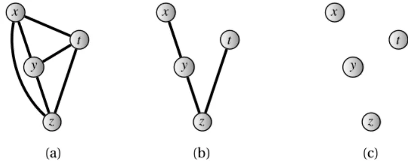
Figure1. Graphical illustrations: (a) full search, (b) partial search, and (c) no search.
alternatives, where she finds a new set of suggested phones. She looks for the best phone within the new suggestions and repeats the process. She stops searching when she finds a phone for which there is no better alternative among those suggested on its page.
Under this strategy, the range of the next search depends only on the best alternative already encountered. We call such a procedureMarkovianCIS. Formally, the decision maker’s consideration set mapping has the structure
(A S)=(∗(xA)∩S)∪A (1)
wherexAis the best item inA,∗is a mapping fromX toK(X), andx∈∗(x). The term∗(x)represents the set of suggested alternatives at the page ofx(the considera- tion set ofx). Sometimes, a suggested item may not be available. Thus, what the con- sumer can actually compare are those items included in the intersection,∗(xA)∩S. We call mapping∗theMarkovian consideration set. We also say that( ∗)represents a Markovian CIScifcis represented by( ), whereis defined by (1). Under the as- sumption that consideration sets are Markovian, we can provide a graphical illustration for the CIS model. InFigure 1, each node corresponds to a particular alternative, and the positions of nodes represent preferences: the higher the position is, the better the alternative is(xtyz). A connection between two alternatives indicates that each of them belongs to the consideration set of the other.10 We illustrate three cases from one extreme to the other with four alternatives inFigure 1(a)–(c): while (a) represents a standard decision maker (independent of starting point, the decision maker considers all feasible alternatives, hence always chooses the best alternative), in (c), she does not consider anything other than the starting point, hence she sticks to the starting point no matter what the budget set is. The interesting case isFigure 1(b): the DM’s best option xis visible fromybut not fromz. Therefore, she cannot reachxwhenzis the starting point unlessy is available. In other words, to choosex, she needs to follow the path z→y→x.
Under the Markovian structure, the search stops whenever the best item so far is also best within its own consideration set. To see this, suppose the decision maker has historyAin whichxis the best element and it is also best in∗(x)∩S. Then her next
10A directed graph can be used to illustrate asymmetric membership of consideration sets: only one of them is the consideration set of the other.
consideration set will beA=(∗(x)∩S)∪A, soxis still the best item. Therefore, her next consideration set is alsoA, so she stops searching and choosesx.
Markovian CIS is a plausible model of search not only for those searching the inter- net, but also for many other scenarios.
• The set∗(x)includes alternatives that have similar attributes or overlapping fea- tures withx, for example, “comps” of a house. It is natural to assume that deci- sion makers who are considering whether to purchase a house compare it only to houses in a similar price range, rather than all available houses.
• Depending on the best item a decision maker has observed so far, some cues (or aspects) of items might look more important than others. The decision maker considers only terms that dominate the current one inthesecues. Hence∗(x) excludes alternatives that incur loss relative toxin any of these cues.
• Depending on trade-offs, some binary comparisons could be difficult. To avoid these difficult trade-offs, the decision maker considers only items that are easy to compare tox.
Characterization
Now, we draw the boundaries for the empirical scope of the Markovian CIS model. To do this, we present a set of postulates that are both necessary and sufficient for Markovian CIS.
The first postulate is a stronger version of theDominating Anchoraxiom, which en- sures the acyclicity of the revealed preference. Given the additional structure of the con- sideration set mapping, the Markovian CIS model generates more revealed preference.
For example, ifx=c({x y} y)butx=c(S y)implies thatxmust be inferior toc(S y) according to the Markovian CIS model, but it may not be in the general CIS model. Thus, we need the following axiom.
A1 (Strong Dominating Anchor). For anyS, there is some alternativex∗∈Ssuch that for anyy∈X, ifx∗=c({x∗ y} y), thenc(T y) /∈S\ {x∗}for allTincludingx∗.
Notice that theDominating Anchoraxiom is the special case ofA1wheny=x∗. If the axiom is violated, then for every alternative inS, there exists another alternative in Sthat is superior. Therefore, the violation of this axiom implies thatSdoes not have a most preferred alternative, which is a contradiction. We discuss the revealed preference of the Markovian CIS model in detail in the next subsection.
The next postulate states conditions under which an alternative is irrelevant for a fixed starting point. An alternative is irrelevant if adding it to a choice set does not affect the choice. First, fix the starting point, say x. If y is irrelevant in {x z}, i.e., c({x z} x)=c({x y z} x), then in the classical choice theory,yis also irrelevant in any decision problem wheneverzis present. In other words, the presence ofzmakesyglob- ally irrelevant. Our next postulate is a weaker version of this idea. For an alternative to be irrelevant globally in the presence ofz, it must be irrelevant in{x z}and it must also dominate the starting point (y=c({x y} x)).
A2 (Irrelevance). Assume y = c({x y} x). Then c({x y z} x) = c({x z} x) implies c(S x)=c(S∪y x)for anySincludingz.
We now illustrate that this is a necessary condition of Markovian CIS. The assump- tions of the postulate imply that bothyandzbelong to the consideration set ofx. Since yis not chosen from({x y z} x),y is never the best element in the first consideration set ifzis available. This means the alternatives encountered in the next stage is the same whetheryis present or not. Hence this postulate is also necessary.
Next, consider a DM who chooses the starting pointxin two different decision prob- lems. The next postulate requires that she also choosesxwhen the two budget sets are combined andxis the starting point.
A3 (Expansion). Ifx=c(S x)=c(T x), thenx=c(S∪T x).
It is easy to see that this is a necessary condition of Markovian CIS. Ifx=c(S x)= c(T x), then there exists no element inSorT such that it is in∗(x)and better thanx.
In this case, the DM sticks to her starting point under the decision problem(S∪T x).
Our final postulate states that if there is only one alternative, sayy, that makes the DM move away from the starting point, sayx, then it does not matter whetherxoryis the starting point. In other words, one can replace the starting point with this dominat- ing alternative.
A4 (Replacement). Ifc(S x)=xandc({x y} x)=y, thenc(S∪y x)=c(S∪y y).
Sincec({x y} x)=y, we must havec(S∪y x)=x. This means the decision maker must encounter a better alternative thanxin the first stage of search. Sincec(S x)=x, there is only one such alternative, which isy. Then she continues to search as if she started fromy because of the Markovian structure. Thus, in both decision problems (S∪y x)and(S∪y y), the DM follows the same path and reaches the same final choice, i.e.,c(S∪y x)=c(S∪y y).11
Theorem2. An extended choice functioncsatisfiesA1–A4if and only ifcis a Markovian CIS.
The proof is provided in theAppendix.
Revealed preference, revealed consideration, and search path
Given that Markovian CIS imposes more structure on the consideration set mapping, we can infer more about the preference of the DM. We now list three choice patterns that reveal the DM prefersxovery.
1. Abandonment of the starting point:x=c(S y).
11In theAppendix, we provide examples to illustrate that these four axioms are independent.
2. Choice reversal:x=c(S∪y z)=c(S z).
3. Chosen over a dominating alternative:x=c(S∪y z)andy=c({y z} z).
The first choice pattern is straightforward. Indeed, the inference thatxis preferred toyis possible when this choice pattern is observed, even when no structure is imposed on the consideration set mapping in the general CIS model.
The second choice pattern is a choice reversal, wherexis unchosen when a seem- ingly irrelevant alternativeyis removed. Then in the decision problem(S∪y z),ymust be the best element at some step of the search process because that is the only way it can affect the DM’s choice. We can conclude thatxis preferred toy because we know thatywas considered andxwas chosen. Notice that this inference is not possible with the general CIS model, in which an element that is not the best at any step may affect the consideration set and thereby influence the final choice.
In the third choice pattern,xis chosen overy, which dominates the starting pointz.
The equalityy=c({y z} z)reveals thatyis inz’s consideration set. Therefore, anything chosen overywhenzis the starting point must be better thany.
Any preference that can representcmust be consistent with the above revelations.
Formally, given a Markovian CISc, let
xcyif one of above three choice patterns is observed
and letTCc be the transitive closure ofc. IfxTCc y, then we can conclude the DM prefersxovery. The converse is also true: any preference that respectsTCc represents cas well. Thus,TCc fully characterizes the revealed preference of the Markovian CIS model. The next proposition states these facts formally.
Proposition1 (Revealed preference). Supposecis a Markovian CIS. Thenxis revealed to be preferred toyif and only ifxTCc y.12
We would like to note that the transitive closure of the binary relation generated by the third choice pattern (chosen over an dominating alternative) itself fully captures the revealed preference of the Markovian CIS model. Thus, the first two patterns (abandon- ing the starting point and choice reversal) may look redundant. For instance, when a choice reversal is observed, one can prove thatxis preferred toy in the sense of the third condition by seeking more choice data and/or applying the axioms to fill in the missing choice data. We provide these two conditions explicitly because it eliminates such a cumbersome requirement and makes Proposition 1more useful for empirical studies.
Now we illustrate when we can conclude thatxis in the consideration set ofy, which we call the revealed consideration set. As in our definition of the revealed preference with multiple representations, we sayxis revealed (not) to be in the consideration set of yif every possible Markovian representation of an extended choice function agrees that xbelongs (does not belong) to the consideration set ofy.
12All results in this section can be easily verified by the proof ofTheorem 2.
To conclude that xis iny’s consideration set, we need to observe x=c({x y} y).
Notice that it is not enough to observex=c(S y)becausexmay be considered only after the DM switches fromy to something else. Alternatively, to inferxis not in y’s consideration set, we need to observey=c(S y)for some S and to know xis better thany. Ifxwere iny’s consideration set, the DM would have abandonedy. The following remarks summarize these observations.
Remark1 (Revealed consideration). Supposecis a Markovian CIS. Thenxis revealed to be in the consideration set ofyif and only ify=c({x y} x).
Remark2 (Revealed inconsideration). Supposecis a Markovian CIS. Then,xis revealed not to be in the consideration set ofyif and only ify=c(S y)for someSincludingxand xTCc y.
Finally, we illustrate what we can infer about the decision making process. For instance, supposec({x y z} x)=y. We may wonder if the DM finds y immediately (in the consideration set of x) or finds y only after inspecting z. If we also observe c({x y} x)=x, we can conclude that the DM findsy only after inspectingz, because this information reveals thaty is not included inx’s consideration set. In this way, we can identify how the DM reachesy, which we call her search path, asx→z→y.
This idea is generalizable. Suppose we would like to know how the DM reaches the final choice in(S x0). We can do so by citing her choice from the set of alternatives that are known to be inx0’s consideration set. If we letS0= {y∈S:y=c({x0 y} x0)}, her next point must bec(S0 x0). Repeating the process, we can fully identify how she reaches her final choice (c(S x0)) from her starting pointx0. Thus, her observed choices fully identify her search path. The following remark formalizes this.
Remark3. Supposecis a Markovian CIS. Every Markovian CIS representation ofcgen- erates the same path for every extended decision problem.
The novelty ofRemark 3is that it provides choice-based insights about the process of search. While the standard search theory informs us of how a DMshould behave, Remark 3tells us how the DM actuallydoesbehave during the search. If the data on the search path are available, our identification result of the search path (Remark 3) can be used to test the model in addition to our axiom.
Some behavioral implications of the Markovian CIS model
The Markovian CIS model retains several consistency properties, even though it accom- modates choice reversal. We highlight the following properties, which are implied by the set of postulates that characterize the Markovian CIS model (Theorem 2).
• Starting Point Bias: Ify=c(S x), theny=c(S y).
• Starting Point Contraction: Ifc(S x)=x, thenc(T x)=xfor allT⊂S.
• Sandwich Property: Ifc(S x)=c({x y} x)=yand{x y} ⊂T⊂S, thenc(T x)=y.
• Irrelevance of Revealed Inferior Alternatives: IfxTCc y, thenc(S x)=c(S∪y x) for allS.
The starting point bias property says that if a decision maker ever choosesy from (S x), then her search outcome will be the same whenyis the starting point. This prop- erty appears as the status quo bias axiom inMasatlioglu and Ok (2005), which interprets the starting point as a status quo. In the Markovian CIS model, the final choice must be best within its own consideration set, and if the DM starts from such an alternative, she will be unwilling to move away.
The starting point contraction property is a version of the independence of irrelevant alternatives (IIA) axiom. This version of the axiom is applicable in the Markovian CIS model when the DM sticks with her starting point, which she does only if she cannot find anything better in its consideration set. If she is happy with her starting point when she faces a large menu, she will still be happy with her starting point when the menu shrinks.
In general, IIA does not apply if the DM does not stick with her starting point.
This is because removing an alternative that is on the path of search can change the DM’s path and cause a choice reversal (Figure 1(b)). Thus, the IIA property is pre- served only when the removed alternative is not on her path of search. For instance, if c(S x)=c({x y} x)=y, then we learn thatyis reached in the initial iteration of search, so all other alternatives inSare off the search path. In this case, we can safely state that removing an alternative (other thanxandy) does not affect the DM’s choice, which is the sandwich property.
The final property—the irrelevance of revealed inferior alternatives property—is based on the observation that an alternative that is worse than the starting point never affects the DM’s search behavior. Taking the unobservability of her preferences into ac- count, this property states that removing an alternative that is revealed to be worse than the starting point does not change her choice.
Additional knowledge about preference and consideration sets
Although we have characterized the Markovian CIS model under the assumption that bothand∗ are unobservable, one can imagine circumstances where these factors are partially or fully observable. In our example of a DM using a website to explore digi- tal cameras, we may learn about consideration sets and thereby observe∗by inspect- ing how the website makes suggestions. In a market with identical products, we may make the reasonable assumption that consumers care only about prices and thereby observe.
To represent a certain extended choice function by the Markovian CIS model, we must use certain pairs of a preference and a consideration set mapping, although they may not be unique. Thus an extended choice function that admits a Markovian CIS
representation may fail to have a representation that is consistent with extra informa- tion about the DM’s preference and consideration sets. We are currently addressing this issue.13
First, consider the case where we fully observe both the DM’s preferenceand the DM’s behaviorc. If she follows the Markovian CIS model, the true preference will not contradict the revealed preference generated byc(TCc byProposition 1). Conversely, if there is no contradiction, we can find a consideration set that maps∗ so thatcis represented by( ∗).14 Thus, as long as there is no contradiction between the DM’s (known) preference and the revealed preference, her behavior can be represented by the Markovian CIS model.
Indeed, this logic is applicable even when we have only partial information about the DM’s preference. For instance, we know she prefersxovery, but do not know how she ranks other elements. In the abstract, we know that her preference must include a partial order (asymmetric and transitive). The special case of full information about the DM’s preference is when is complete. The following remark summarizes these findings and can be easily verified by the proof ofTheorem 2.
Corollary1. Letcbe an extended choice function and letbe a partial order overX. Then there exists a pair of preferenceand Markovian consideration set mapping∗that representsc, andxywheneverxy, if and only if (i)csatisfiesA1–A4and (ii)does not contradictTCc (there is noxandysuch thatxybutyTCc x).
Next, we study the case where the consideration set is fully observable to be ∗. Unlike the known preference case, the consistency between revealed (in)consideration and ∗ is not sufficient for a valid representation. The first extra condition we must impose is that the DM never moves away from her starting point if we know that she does not consider anything other than her starting point.
The second condition is about the consistency of the revealed preference gener- ated by this extra information. Suppose we observex=c(S z) and it is known that y∈∗(z).15 Then clearly the DM’s final choice is made after consideringy, so we learn thatxis preferred toy. Formally, for any distinct alternativesxandy,
xcyif and only ifc(S z)=xfor somezandSywithy∈∗(x)
where the possibility ofz=yis not excluded. Notice that the revealed preferencec
due to the extra information about∗(x)contains more information than the revealed preferencec generated without this information. It happens thatz=c({y z} z)and thaty∈∗(z)is known. Thus, the slightly stronger revealed preference must not have a contradiction.
13Cherepanov et al. (2013)andManzini et al. (2011)also study a similar question in different contexts.
14We showed this in the proof ofTheorem 2. We can take any completion ofcas the preference to represent a given choice function.
15As we have seen, ify=c({y z} z), thenxyis revealed even without the extra information about∗, because that choice itself revealsy∈∗(z).
It turns out that these two extra conditions, along with all of the axioms inTheo- rem 2, are sufficient for an extended choice function to be compatible with the Marko- vian CIS model. The proof is given in theAppendix.
Proposition2. Letcbe an extended choice function and let∗be a Markovian consid- eration set mapping. Then there exists a preferencesuch that( ∗)representscif and only if
(i) csatisfiesA1–A4
(ii) if∗(x)∩S= {x}, thenc(S x)=x (iii) chas no cycle.
4. Unobservable starting points
Our revealed preference approach is based on the assumption that we can observe not only what the decision maker chooses from a budget set, but also which alternative she initially contemplates. However, we can also imagine situations where we observe only standard choice data and do not observe the starting point. For example, if the starting point is what the DM expects to buy in the market, it can be difficult to elicit such infor- mation. Given possible limitations in the data, we investigate how to identify DM’s who follow an underlying CIS model (general or Markovian).
Suppose the DM actually follows a CIS model denoted byc, but we do not observe her starting point. We observe her choosingy fromS—the only available data. Then there must exist a starting point that leads her to picky. Of course, such a starting point may not be unique; several distinct starting points might result in the same final choice, y=c(S x)=c(S z). At the same time, given a fixed budget set, observed final choices might depend on the starting points,y=c(S x)andw=c(S z). We definethe choice correspondence inducedbyc, denoted byCc:K(X)→K(X), as
y∈Cc(S)if there existsxsuch thaty=c(S x)
In other words,y∈Cc(S)meansyis chosen fromSfor some starting point. This is in line withSen (1993): “It may be useful to interpretC(S)as the set of ‘choosable’ elements—
the alternatives that may be chosen.”16 Note thatx y∈Cc(S)does not imply thatxis indifferent toy in our framework. It simply means that bothxandy may be chosen fromS, depending on the starting point.
The induced choice correspondence,Cc, is what one can observe when the DM fol- lows a particular CIS,c, but her starting point is unobservable. In other words,Cc are the only available data to an outside observer who knows that the choices of the DM are affected by the starting point but lacks information about the starting point.
16Salant and Rubinstein (2008)also follow this idea in defining a choice correspondence from a frame- dependent choice function.
General model
We first start with the general model. Imagine that we observe a choice correspon- dence C. We would like to determine if there exists a general CIS model, sayc, that induces the observed choice correspondence, i.e., C=Cc. Such a general CIS model exists if and only if the DM’s choice correspondence satisfies a simple axiom called the Bliss Pointaxiom. This result makes it possible to identify DM’s following a CIS even with standard choice data.
TheBliss Point Axiom(BP). For any setS, some may-be-chosen alternative fromS must always be may-be-chosen from any smaller decision problem: There existsx∈C(S) such thatx∈C(T )ifx∈T⊂S.17
We call the alternative that satisfies the condition of BP a bliss point ofS. By con- trast, IIA dictates thatall may-be-chosen alternatives should be may-be-chosen from any smaller choice problem (whenever they are available). Therefore, BP relaxes IIA by requiring thatonemay-be-chosen element fulfills the condition rather than all may-be- chosen elements. Even though BP is a weaker condition than IIA, it still does not allow choice cycles.
We next show that BP guarantees the existence of underlying choice by iterative search.
Proposition3. A choice correspondenceC satisfies theBliss Pointaxiom if and only if there exists an underlying CIS that inducesC.
The power ofProposition 3is that it connects choice patterns that are considered
“irrational” in traditional choice theory to our choice by iterative search model, which captures bounded rationality. It provides a very simple and intuitive postulate to identify CIS decision makers using only choice data.
Markovian
We would like to reconsider the case where our data are limited to the choices from a choice set—there is no knowledge about starting point. As before, we would like to identify DM’s who follow an underlying Markovian CIS from such restricted data. If a choice correspondenceCis generated by an acyclical binary relation,18then there exists an underlying Markovian CIS that inducesC.
Proposition 4. A choice correspondenceC can be rationalized by an acyclical binary relation if and only if there exists an underlying Markovian CIS that inducesC.19
17This axiom appears inAgaev and Aleskerov (1993)as “the fixed-point condition” to characterize inter- val choice models.
18We say that a choice correspondenceCis generated by an acyclical binary relationPifC(S)= {x∈S| there exists noysuch thaty P x}.
19When the starting point is not observable, the Markovian CIS model is observationally equivalent to K˝oszegi and Rabin’s (2006) personal equilibrium, which is also generated by an acyclic preference as shown byGul and Pesendorfer (2006).
This provides a very simple test of Markovian CIS using only limited data. In ad- dition,Proposition 4makes it possible to identify behavior that is consistent with the general model but not with the Markovian model, even absent data on starting points.
Therefore, standard choice data alone are enough to make the distinction between the general and the Markovian CIS models.
Finally, we discuss how and to what extent one can infer the preference of the DM following the Markovian CIS model from this limited data. First, let us clarify what a revealed preference means in this context. Since multiple Markovian CIS models can generate the same choice correspondenceC, naturally we definexto be revealed pre- ferred toyif and only if the preference of every Markovian CIS model generatingCranks xabovey. The proof ofProposition 4shows that any completion of the acyclical bi- nary relation rationalizingC represents one of Markovian CIS models generatingC(by choosing∗appropriately). Therefore, the transitive closure of this relation is the full characterization of the revealed preference in this context.
5. Related literature
CIS is related to three branches of decision theory: search, limited consideration, and reference dependence. We discuss the relationships of both the general CIS model and the Markovian CIS model to these branches.
Search
Caplin and Dean (2011) also study search by employing the revealed preference ap- proach. Their model also assumes decision makers have a stable preference. They utilize a different type of auxiliary data calledchoice process data. These data include what the decision maker would choose at any given point in time if she were suddenly forced to quit searching. The entire path followed during the course of search is the in- put of their model, rather than its output. The novelty of our approach is that the path of interim choices (the choice process data) can be uniquely identified by imposing cer- tain structures—such as that considered in our Markovian CIS model—on consideration sets.20
Limited consideration
In the recent literature on limited consideration, a DM chooses the best alternative from a small subset of the available alternatives. In contrast to the CIS model, most of them focus on some aspects of decision making other than searching. For instance, in many models of limited consideration, the DM, prior to choosing the most preferred element, applies some criteria other than her preference to theentire feasible set to eliminate
20Papi (2012),Horan (2010), andRaymond (2011)also analyze choice as a process of search. All of these papers assume that the order of search is part of the decision problem and is observable to the analyst. In contrast, in our approach the order of search (except the starting point) is in the mind of the decision maker and is unobservable to the analyst.
some alternatives. Such models include the rational shortlisting (Manzini and Mari- otti 2007), considering only alternatives that belong to the best category (Manzini and Mariotti 2012) and considering only alternatives that are optimal according to some ra- tionalizing criteria (Cherepanov et al. 2013). These procedures cannot be implemented without knowing the entire feasible set, so these models are inconsistent with an envi- ronment where the DM must find her alternatives through search.
Salant and Rubinstein (2008)study a decision making process in which the DM con- siders only the topnelements according to some ranking and chooses her most pre- ferred element from that restricted consideration set. The model is consistent with a search environment if the ranking is, for instance, the amount of advertising for an ele- ment, because limited consideration arises even when the DM is unaware of the entire feasible set. However, this procedure assumes that she is following a fixed stopping rule and she does not adjust her search strategy during the search process.
Masatlioglu et al. (2012)provide a model of limited attention, where the considera- tion set depends only on the budget set, denoted by(S). Unlike the CIS model, their model is agnostic about how such a consideration set is formed. Instead, they impose a condition that is satisfied in many environments and procedures. The condition says that the consideration set is unaffected by removing an alternative that does not attract attention:x /∈(S)implies(S)=(S\x). The final consideration set generated by the Markovian CIS model (fixing the starting point) satisfies this property.21 Thus, one can viewMasatlioglu et al. (2012)as a reduced-form model. where one of the possible un- derlying structures is CIS. Nevertheless, the strong structure of the Markovian CIS model makes it possible to identify more preferences than the limited attention model in the sense of set inclusion. InSection 3, we illustrate three types of choice patterns that re- veal the DM’s preference, whereas only choice reversal does so in the limited attention model.
Reference dependence
The CIS model is also related to the literature on reference-dependent preferences. In particular, the Markovian CIS model captures dynamic adjustments of the reference point in search, where the reference point at any given stage is the best element in the current consideration set. Each reference point restricts the set of options the DM is willing to currently consider. The DM continues to adjust her reference point until the current reference point is the best within its consideration set. Previous models of reference-dependent choices such asTversky and Kahneman (1991),Masatlioglu and Ok (2005), andSalant and Rubinstein (2008)are static—the reference point is exoge- nously given and fixed.
Tversky and Kahneman (1991) introduce the first reference-dependent model, where losses have a greater impact than corresponding gains on utility (loss aversion).
Their loss aversion model allows strict cycles: a DM strictly prefersytoxwhen endowed with x, strictly prefers z toy when endowed with y, and strictly prefersxto z when
21We should note that the final consideration set generated by the general CIS model might not satisfy this property, hence their model is more restrictive than our general CIS model.
endowed withz, i.e., xzzy yxx. In the CIS model, the reference point is aban- doned only when there is a welfare improvement, so their model is not a special case of the CIS model. Unlike the DM in this reference-dependent model, the DM in the CIS model can violate IIA, even for a fixed starting point. Therefore, these two models are independent.22
Masatlioglu and Ok (2005)propose a reference-dependent choice model, where a DM follows a simple two-stage procedure: elimination and optimization. In the elimi- nation stage, the DM discards all alternatives other than those that dominate the status quo (sayr) in every (endogenously driven) aspect. Formally, the set of surviving alter- natives inSis{x∈S|ui(x)≥ui(r)for alli} ∩S, whereuirepresents the ranking in as- pecti. In the optimization stage, the DM simply chooses the best alternative from the set of surviving alternatives. For comparison purposes, we interpret the set of the alter- natives that can survive over the status quorto be the consideration set ofr, denoted by∗(r). Thus, the DM’s choice fromS is the best alternative in∗(r)∩S. The first difference between models is that inMasatlioglu and Ok’s (2005) model, decisions are made just after the first round (static), whereas the final consideration set dynamically involves the Markovian CIS model. In addition, because of the multi-utility representa- tion,Masatlioglu and Ok’s (2005) consideration set enjoys a nested structure:x∈∗(y) implies∗(x)⊂∗(y), which is not imposed in the Markovian CIS model.
However, the difference between the two models disappears when we also impose the nested structure on the consideration set of the Markovian CIS model. This is because once the DM finds the best element in the consideration set of the starting point, she will not find any more new alternatives in the next consideration set given the nested structure, so she stops searching immediately, which is behaviorlly equiva- lent toMasatlioglu and Ok’s (2005) model. Thus, the difference is solely generated by Masatlioglu and Ok’s (2005) particular structure of the consideration set driven by the multi-utility representation.
Masatlioglu and Ok (2010)provide a more general version of the status quo bias model by eliminating the nested structure on∗. Given the behavioral equivalence be- tweenMasatlioglu and Ok (2005)and the Markovian CIS model with the nested struc- ture, one may suspect thatMasatlioglu and Ok’s (2010) model is equivalent to the Marko- vian CIS model without any particular structure on∗. However, the static nature of the status quo model now makes these two models distinguishable. Letxbe the best al- ternative within∗(r). UnlikeMasatlioglu and Ok’s (2005) model, it is possible that the consideration set ofxcontains something better thanx. Nevertheless,Masatlioglu and Ok’s (2010) DM simply picksx, while the Markovian CIS’s DM continues searching. In- deed, the model inMasatlioglu and Ok (2010)does not allow choice reversals for a fixed status quo, but the Markovian CIS does. Conversely, the Markovian CIS model satisfies the following condition: ifc(S x)=y, thenc(S y)=y, which is not implied by their model. In sum, the status quo bias models and the Markovian CIS model are only be- haviorally equivalent when the consideration set or the set of surviving alternatives has the nested structure, but this is not the case in general.
22Since the model ofK˝oszegi and Rabin (2006)is closely related toTversky and Kahneman (1991), these differences also apply to their formulation of reference dependence.
Salant and Rubinstein (2008)study choices in the presence of a framing effect using the(A f )model, which is the most general reference-dependent choice model. A frame f is irrelevant in the rational assessment of alternatives, but nonetheless affects choice.
The CIS model can be thought of as a special case of the (A f )model by letting the frame be the starting point.
6. Concluding remarks
We recognize that people must engage in a dynamic process to learn about feasible al- ternatives, especially in complicated decision problems such as searching for a house.
Thus, we incorporate the idea of search and consideration sets into decision theory to get new insights into how people make decisions in such circumstances.
We illustrate how to infer a DM’s preference and search process from the choice data in the Markovian model. The choice data partially distinguish the DM’s preference and consideration sets. This is useful for firms. For instance, if a product is unpopular, it is important for a firm to know why. Is it because consumers do not like the product or because they cannot find the product in the course of their search? These identification results can help firms identify the reason and react accordingly.
We mention two interesting future directions to explore. The first one is to study the implications of the CIS model using extended market share data (such as 40% of con- sumers starting fromxend up choosingy) rather than extended individual choice data.
With such limited data, we cannot observe how each individual reacts when the feasi- ble set or the starting point changes; we can only observe reactions at the aggregated level. Then a reasonable question is how to identify thedistributionsof preferences and consideration sets if each individual follows a Markovian CIS model.
The second direction is to study the effect of framing on consideration sets. While most of our work makes the useful simplification that consideration sets are affected only by the history and the feasible set, one could consider cases where consideration sets are affected by more general framing effects (such as presentation and advertising).
In these cases, the consideration set can be written as(A S f )or∗(x f ), wheref is a frame.
Appendix
A.1 Independence ofA1–A4
The following examples illustrate that, in our characterization for the Markovian model, no axiom can be disposed without affecting the characterization. We drop each axiom, one at a time, in their numerical order.
• If the consideration set mapping,∗, is allowed to depend on the starting point, one can create examples whereA1is violated and the rest of the axioms are satis- fied.
• If the pair( ∗)is allowed to depend on the composition of the budget set, one can create examples whereA2is violated and the rest of the axioms are satisfied.
• Consider a decision maker who stays with her status quo except once (c(X x)= y=x). This example violatesA3and satisfies the rest of the axioms.
• If one modifies the model and considers the one-step-limited search model (search terminates after the first step, i.e.,c(S x)=arg max( ∗(x)∩S)), this model satisfiesA1–A3, but violatesA4.
A.2 Proof ofTheorem 2
The proof of the “if” part is left to readers. Now suppose c satisfiesA1–A4. For any distinctxandy, definexandy:
xcyifx=c(S z)andy=c({y z} z)for somez=xandy∈S Notice that this definition does not exclude the possibility thatyis equal toz.
We now show thatA1guarantees thatcis acyclical. AssumecsatisfiesA1andcis cyclic. If elements ofSform a cycle in terms ofc, this means that for every alternative x∈S, there existzxandy∈S\ {x}such thatc({x zx} zx)=xandy=c(T zx)for some (T z), which violatesA1. Hence,ccannot have a cycle.
Sincecis acyclical, we can find a strict rankingthat includesc. Define∗(x)≡ {y|c({x y} x)=y}and note that x∈∗(x)for all xinX. Then( ∗) generates a Markovian CIS. Let us denote it byc∗: we will show thatc∗=c. First, we need to prove several claims.
Claim1. Ifc(S x)=x, thenc(T x)=xwheneverT ⊂S.
Proof. Assumec(S x)=x=c(T x)andT⊂S. ByA3, there existsz∈T \xsuch that c({x z} x)=z. By applyingA4,c(S x)=xandc({x z} x)=zimplyc(S∪z x)=c(S∪ z z). Sincezalso belongs toS(⊃T), thenc(S x)=c(S z). Hencec(S z)=x, andA1is
violated because ofc(S z)=xandc({x z} x)=z.
Claim2. We have∗(x)∩S= {x}if and only ifc(S x)=x.
Proof. The equalityS∩∗(x)= {x}implies thatx=c({x y} x)for ally∈S. Then, by A3, we havec(S x)=x. Alternatively, ifc(S x)=x, then, byClaim 1,x=c({x y} x)for
ally∈S. HenceS∩∗(x)= {x}.
Claim 3. Let x=y. Then c(S x) =c({x y} x) =y and ∗(x)∩S = {x y} implies c(T x)=ywhenever{x y} ⊂T⊂S.
Proof. ByA3, it isc(T\y x)=xbecausec({x z} x)=xfor any z∈T\y by con- struction of ∗ for any T ⊂S. Together with c({x y} x)=y, we can, in particular, get c(S y)=c(S x)=y and c(T y)=c(T x) by A4. The former andClaim 1 imply
c(T y)=y, so it must bec(T x)=y.
Claim4. Letx y z∈Sbe all distinct alternatives. Ifc(S x)=c({x y} x)=y andz∈ ∗(x), thenc(T x)=c(T \z x)for anyT includingxandy.
Proof. By construction of∗, we havez=c({x z} x), so we can get the desired result by provingc({x y z} x)=yso thatA2is directly applicable. First note thatc({x y z} x) cannot be x because of Claim 2 (notice that y z∈∗(x)). To see why it cannot be z, if it were, it must bec({x y z} x)=c({x z} x)=z by A2and z ∈∗(x). Thus, it must bezcy. Alternatively,c({x z} x)=zandc(S x)=y requireycz, which is a
contradiction.
Claim5. Letx=y. Thenc(S x)=c({x y} x)=yimpliesc(T x)=ywhenever{x y} ⊂ T⊂S.
Proof. LetQ=(∗(x)\ {x y})∩S. By applyingClaim 4repeatedly,c(T\Q x)=c(T x) andc(S\Q x)=c(S x)=y. SinceT\Q⊂S\Qand(S\Q)∩∗(x)= {x y},Claim 3
requiresc(T \Q x)=y. Hence,c(T x)=y.
Claim6. Ifxy, thenc(S x)=c(S∪y x).
Proof. Let
D= {(x y S)|xyandc(S x)=c(S∪y x)}
Dmin= {(x y S)∈D| there is no(x y S)∈DandSS}
We show thatDminis empty. ThenDmust be empty as well, which is the statement of Claim 6.
Observation1. If(x y S)∈D, then (i)c(T x)=yfor anyT, (ii)c({x y} x)=x, (iii)x, y,c(S x),c(S∪y x)are all distinct, and (iv)c({x c(S∪y x)} x)=x.
Proof. (i) If not, we haveycx, which contradictsxy.
(ii) This is just a special case of (i) whenT= {x y}.
(iii) If eitherc(S x)orc(S∪y x)is equal toy, it contradictsxy. Ifx=c(S x), by (ii) andA3, we havex=c(S x)=c(S∪y x), a contradiction. Ifx=c(S∪y x), by Claim 1, we havex=c(S x)=c(S∪y x), a contradiction.
(iv) Ifc({x c(S∪y x)} x)=c(S∪y x), byClaim 5, we havec(S x)=c(S∪y x), a
contradiction.
Observation2. If(x y S)∈Dmin, there exists uniquet∈S\xsuch thatc({x t} x)=t.
Proof. Existence: Suppose there is no sucht. Thenc(S x)=xbyA3, which is a con- tradiction (Observation 1(iii)).
Uniqueness: Suppose that there is another elementt∈S\xsuch thatc({x t} x)= t. Thenc({x t t x} x)=xbyClaim 2. Without loss of generality, letc({x t t} x)= c({x t} x)=t. Then byA2,c(T x)=c(T ∪t x)whenevert∈T. In particular, we have c(S\t x)=c(S x)andc(S∪y\t x)=c(S∪y x). Sincec(S x)=c(S∪y x), we have c(S\t x)=c(S∪y\t x). Thus,(x y S\t)∈D, which contradicts(x y S)∈Dmin.
Observation3. If(x y S)∈Dmin, and we letz=c(S x)andz=c(S∪y x), then there existsw∈S\zsuch that(w y S)∈Dmin,c({w z} w)=z,z=c(S w), andz=c(S∪y w).
Proof. The easy case: Ifz=c({x z} x), then letw=x.
The difficult case: Supposex=c({x z} x). ByObservation 2,S\xhas only one el- ementtsuch thatt=c({x t} x). Thus,A3impliesc(S\t x)=x, soc(S x)=c(S t)by A4. Similarly, we getc(S∪y x)=c(S∪y t)becausec({x y} x)=xbyObservation 1.
Therefore, we havez=c(S t)=c(S∪y t)=z. Furthermore, it must be thattybe- causetcxy. Hence,(t y S)∈Dmin. ApplyingObservation 1(iii), it must be thatt=z sot=c({x t} x)andz=c(S x)implieszct. Thus, it must be thatztx.
Ifz=c({t z} t), then letw=t. Ift=c({t z} t), repeating this argument (the dif- ficult case), we can find anothert∈S\xsuch that(t y S)∈Dmin and ztt. If t=c({t z} t), repeat this process. Each time, we find a better alternative than the pre- vious one, so this case cannot be repeated forever. At some point, we must go to the easy
case.
Given these observations, we complete the proof of the claim. Suppose(x y S)∈ Dmin andz=c(S x), z=c(S∪y x). Letw be the element satisfying the conditions in Observation 3. By Observation 1 and Observation 2, c({w z} w)=z (=w) and c({w w} w)=wfor allw∈S\z. Together withc({w y} w))=w,A3impliesc(T w)=w for anyT ⊂S∪y, so it must bec(T w)=c(T z)byA4. In particular, considerT =S, S∪y, and{w y z}. Then we havec(S z)=c(S w)=z,c(S∪y z)=c(S∪y w)=z, and c({w y z} z)=c({w y z} w). ByClaim 2,c({w y z} w)is notwbecausec({w z} w)= z and is noty becausewy, so it isz. ApplyingA3to the first and the third, we get
c(S∪y z)=z, which is a contradiction.
We next define the concept of replacement of a dominated starting point. That is, ifyis a replacement ofxatS, then (i) the DM will reach the final choice in both deci- sion problems(T x)and(T y)for all subsets ofS, including bothxandy, and (ii) any alternative in∗cannot be chosen when the starting point isy. The formal statement follows.
Definition 1. Supposec(S x)=x. Theny∈S\xis called a replacement of xatS if and only if (i)c(T x)=c(T y)for anyT such that{x y} ⊂T ⊂Sand (ii) for anyz∈Sif c({x z} x)=z, thenc({y z} y)=y.
Claim7. Any replacement ofxatSbelongs to∗(x).
Proof. Letybe one of the replacements ofxatS. Definition 1(i) implies thatc({x y} x)=c({x y} y). Substitutingz=xintoDefinition 1(ii) says that ifc({x x} x)=x(al- ways true), thenc({x y} y)=y. Hence, it must be thatc({x y} x)=y, i.e.,y∈∗(x).
Claim8. Supposec(S x)=x. Thenc(S∩∗(x) x)is the unique replacement forxinS.