Relaxing Box Constraints for Systems of Linear Equations
Kiyoshi Yoneda
∗Masahiro Abiru
†Mathias Bosset
‡Abstract This note proposes a method to relax box-type constraints to systems of linear equations in such a way that if a solution exists within but somewhat away from the box boundaries then an optimal solution is obtained, otherwise a best possible alternative outside the box can be found. This is a straightforward application of the principle of embedding which observes that if a solution of an unconstrained optimization satis- fies the constraints, then it is a solution of the corresponding constrained optimization. No extra parameter input is required, which is convenient for applications.
Keywords: inverse problems, simultaneous equations, opti- mization
∗Fukuoka University, [email protected]
†Fukuoka University, [email protected]
‡Fukuoka University, [email protected]
−377−
( 1 )
1 Introduction
Consider solving a system of linear equations in reals Xθ≈z
⎡
⎢⎢
⎢⎢
⎢⎢
⎢⎢
⎣
1 0
. ..
0 1
...
· · · Xij · · · ...
⎤
⎥⎥
⎥⎥
⎥⎥
⎥⎥
⎦
⎡
⎢⎣ ... θj
...
⎤
⎥⎦≈
⎡
⎢⎣ ... zi
...
⎤
⎥⎦ (1)
with respect to θ, where “≈” is for approximate equality. The top identity submatrix of X means that in the input-output relationship X : θ → z the input is a part of the output: the action itself is a part of its consequence. Since X has more rows than columns, no solution may be expected to exist in the sense of linear algebra.
Such problems are in practice often box-constrained in the sense that a solution is desired to be found within a hyperbox:
people usually know a reasonable interval in which a value is to be expected. To simplify notation we let
∀i 0< zi <1 (⇒ 0< θj < 1) (2) without loss in generality. Note that the lower, nonidentity part of X is unbounded; the feasibility is not guaranteed.
Define a “distance” f(xi, zi) where f is convex in xi . Then a solution to (1) may be defined to be
θˆ:= arg min
θ∈]0,1[
i
wif(xi, zi), x:=Xθ (3)
−378−
( 2 )
wherewi are importance weights for the equations. A proposal [2] has been to take
fz(x) := f(x, z) := x
z −1
logx z +
1−x 1−z −1
log1−x
1−z (4) which will be referred to as an (individual) loss function.
An inconvenience with this approach is that a feasible so- lution, which would serve as a starting point for successive improvement, may be nonexistent or difficult to find. The pur- pose of this note is to remove this inconvenience by relaxing the constraints in such a way that:
If a feasible solution exists within (but somewhat away from) the box boundaries then that will be found; otherwise an infeasible alternative (which is best in a way) will be found.
The idea is to use the principle of embedding which simply observes that:
If a solution of an unconstrained optimization sat- isfies the constraints, then it is a solution of the corresponding constrained optimization.
Assume that there is a vector oftolerances0< u such that z and z±u are indistinguishable to the decision maker, the user of the solution. Now extend the loss function in such a way that it equals (4) within ]u,1−u[ := Π ]ui,1−ui[ and quadratic beyond that box. Then this extended loss function is indistinguishable to the user from the original (4) but is actually defined over the entire space, accepting any initial so- lution. If the derivatives, up to second, of the extended loss
Relaxing Box Constraints for Systems of Linear Equations(Yoneda・Abiru・Bosset) −379−
( 3 )
match those of the original loss atu and 1−u, then Newton’s method works and the minimization in (3) converges quadrat- ically. The solution thus obtained matches that of the original problem if it exists within the box ]u,1−u[ and, if it exists outside the box, still provides the best infeasible solution.
In section 2 the original loss function in the interval ]0,1[
is briefly reviewed. Section 3 extends the loss function beyond the interval. Section 4 points out that the weights to the linear equations in (1); viz.,wi can be derived from ui, meaning that there is no labor involved in setting up the extra parameters.
The final section 5 remarks on a possible application to knowl- edge representation. The Appendix includes some programs in R.
2 Loss function within the box
From this section and on the subscriptsiandj forXij will be dropped when clear since we’ll be talking mainly about fz(x) . The loss function within ]u,1−u[, 0< u < 12 and its first and second derivatives are:
fz(x) = x z −1
logx
z +
1−x 1−z −1
log1−x 1−z dfz(x)
dx = 1 x
x z −1
+ 1
zlogx z− 1
1−x
1−x 1−z −1
− 1
1−z log1−x 1−z d2fz(x)
dx2 = 1 x
1 x + 2
z
+ 1
1−x 1
1−x + 2 1−z
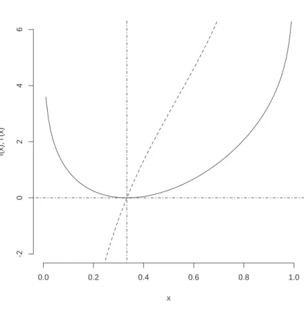
They are illustrated in Figures 1 and 2.
−380−
( 4 )
0.0 0.2 0.4 0.6 0.8 1.0
-20246
x
f(x), f'(x)
Figure 1: The loss function
The loss function (solid) forz = 13 (vertical dot- dash) with its derivative (dashed).
Relaxing Box Constraints for Systems of Linear Equations(Yoneda・Abiru・Bosset) −381−
( 5 )
0.0 0.2 0.4 0.6 0.8 1.0
020406080100
x
f"(x)
Figure 2: The second derivative For the same loss function in Figure 1.
−382−
( 6 )
3 Extension beyond the box
To find a quadratic function to extend the loss function beyond the box, let
c0+c1x+c2x2= fz(x) c1+ 2c2x= fz(x) 2c2= fz(x) to find
c2= 1 2fz(x) c1= fz(x)−2c2x
c0= fz(x)−c1x−c2x2 . To summarize, the extended loss function is
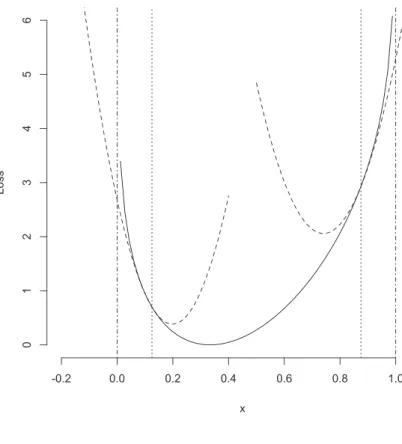
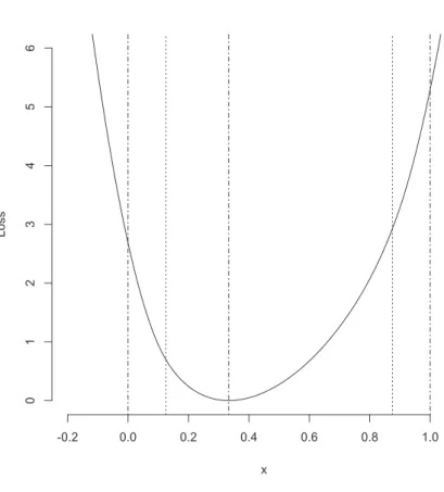
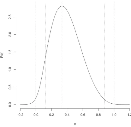
z(x) :=fz(x) x∈]u,1−u[ (5) c0+c1x+c2x2 otherwise (6) illustrated in Figures 3 and 4. Observe that13(1)< 13(0): the solution encontered outside ]0,1[ is more likely to be negative than to exceed one. The corresponding Gibbs distribution ∝ exp{−13(x)}in Figure 5. Note that the resulting tail parts are as with the normal distribution.
The problem (3) may be solved directly and quickly by Newton’s or other methods, but it is possible to regard the set- ting as a generalized linear modelto solve it with the standard iteratively reweighted least squares algorithm, in which case the link function is as in Figure 6 and the mean function or the inverse link function is as in Figure 7.
Relaxing Box Constraints for Systems of Linear Equations(Yoneda・Abiru・Bosset) −383−
( 7 )
-0.2 0.0 0.2 0.4 0.6 0.8 1.0
0123456
x
Loss
Figure 3: The quadratic extension
The loss function (solid) 13(x) for u= 18 (ver- tical dotted), extended quadratically (dashed) left and right forx < 18 and 1−18 < x, respectively.
−384−
( 8 )
-0.2 0.0 0.2 0.4 0.6 0.8 1.0
0123456
x
Loss
Figure 4: The extended loss function
13(x) =f1
3(x) x∈
1 8,7
8 c0+c1x+x2x2 otherwise.
Relaxing Box Constraints for Systems of Linear Equations(Yoneda・Abiru・Bosset) −385−
( 9 )
-0.2 0.0 0.2 0.4 0.6 0.8 1.0 1.2
0.00.51.01.52.02.5
x
Figure 5: The corresponding Gibbs distribution
∝exp{−13(x)}}.
−386−
( 10 )
-3 -2 -1 0 1 2 3
-0.20.00.20.40.60.81.01.2
y
g(y)
Figure 6: The link function
Relaxing Box Constraints for Systems of Linear Equations(Yoneda・Abiru・Bosset) −387−
( 11 )
-0.2 0.0 0.2 0.4 0.6 0.8 1.0 1.2
-3-2-10123
g(y)
y
Figure 7: The mean (inverse link) function
−388−
( 12 )
4 Deriving weights from tolerance
This section points out thatwmay be derived fromu, meaning there is no work for the user involved in setting extra parame- ters. This is of practical importance in applying the method.
A convenient way to set u is to consider how many digits are effective in y. If the value of y should be respected to di digits or 10−d, then y may be considered to be uniformly distributed over y ± 12 ×10−(d+1). Thus 10−(d+1) ∝ si, the standard deviation ofy. Hence u∝s may be used to set
wi ∝ 1 u2i
wi = 1 .
5 Concluding remarks
The extension (6) is by no means the only possibility. The major requirements to the extension are:
• the extended loss is defined over the real,
• the 0th to the 2nd derivatives of at x= umatch those of f,
• the Gibbs distribution ∝ exp −z(x) indeed defines a probability density function, and
• some empirical justification is available.
Most any is permissible so long as the above conditions are met.
Since the version proposed in this note has tails correspond- ing to the normal distribution, it is valid if the outliers which
Relaxing Box Constraints for Systems of Linear Equations(Yoneda・Abiru・Bosset) −389−
( 13 )
fall outside of ]0,1[ are due to various small factors added up.
Now if the outliers are produced not that way but by signal noise or transcription errors, a fatter tail distribution would be more appropriate as a model. In such a case a suitable loss function may be defined in various ways, but not as simply as the present proposal.
The problem described by (1) and (2) is general enough for a wide variety of applications. One which might be worth considering is a box-constrained version ofstructural equations modeling. The input to the agent isθ, its output isyor a part of it. A new piece of knowledge is introduced as a new equation included into the system of linear equations. An immediate problem to deal with in this direction is the inclusion oflatent variables.
References
[1] R Development Core Team. R: A Language and Environ- ment for Statistical Computing. R Foundation for Statisti- cal Computing, Vienna, Austria, 2010. ISBN 3-900051-07- 0.
[2] K. Yoneda. A loss function for box-constrained inverse problems.Decision Making in Manufacturing and Services, 2(1–2):79–98, 2008.
Appendix
The loss function definitions in R [1] and link and mean func- tion implementations are included.
−390−
( 14 )
# original loss
xb.loss.m <- function(x,z=1/3){
r <- x/z; s <- (1-x)/(1-z) ((r-1)*log(r)+(s-1)*log(s))}
xb.loss.m.1 <- function(x,z=1/3){
r <- x/z; s <- (1-x)/(1-z)
((1/x*(r-1) + 1/z*log(r)) - (1/(1-x)*(s-1) + log(s)))}
xb.loss.m.2 <- function(x,z=1/3){
(1/x*(1/x + 2/z) + 1/(1-x)*(1/(1-x) + 2/(1-z)))}
# quadratic
c2 <- function(x,z=1/3){xb.loss.m.2(x,z)/2}
c1 <- function(x,z=1/3){xb.loss.m.1(x,z) - 2*c2(x,z)*x}
c0 <- function(x,z=1/3){xb.loss.m(x,z) - c1(x,z)*x - c2(x,z)*x^2}
quadratic <- function(x,z=1/3){
a0 <- c0(x,z); a1 <- c1(x,z); a2 <- c2(x,z) function(y){a0 + a1*y + a2*y^2}}
# extended loss
xbox <- function(z=1/3,u=1/8){
qx.l <- quadratic(u,z) qx.r <- quadratic(1-u,z) function(x){
ifelse(x<u,qx.l(x),
ifelse(1-u<x,qx.r(x),xb.loss.m(x,z)))}}
Relaxing Box Constraints for Systems of Linear Equations(Yoneda・Abiru・Bosset) −391−
( 15 )
# link function
lf <- function(y,z=1/3,u=1/8){
lf1 <- function(y,z=1/3,u=1/8){
xb.loss <- xbox(z,u)
f <- function(x){y^2-xb.loss(x)}
l <- ifelse(y<0,-0.5,z) u <- ifelse(y<0,z,1.5) uniroot(f,c(l,u))$root}
a <- c()
for (i in 1:length(y))
{a <- c(a,lf1(y[i],z,u))}
a}
# mean function = inverse link function mf <- function(x,z=1/3,u=1/8){
mf1 <- function(x,z=1/3,u=1/8){
xb.loss <- xbox(z,u)
f <- function(y){y^2-xb.loss(x)}
l <- ifelse(x<z,-5,0) u <- ifelse(x<z,0,5)
uniroot(f,lower=l,upper=u)$root}
a <- c()
for (i in 1:length(x))
{a <- c(a,mf1(x[i],z,u))}
a}
−392−
( 16 )