Studies on Data-Driven Controller Tuning for Cascade Control Systems

Studies on Data‑Driven Controller Tuning for Cascade Control Systems

著者 グエン クアン フィ

著者別表示 Nguyen Quang Huy journal or

publication title

博士論文本文Full 学位授与番号 13301甲第4623号

学位名 博士（工学）

学位授与年月日 2017‑09‑26

URL http://hdl.handle.net/2297/00054252

Dissertation

Studies on Data-Driven Controller Tuning for Cascade Control Systems

Graduate School of

Natural Science & Technology Kanazawa University

Division of Electrical Engineering and Computer Science

Student ID No.: 1424042015

Name: Nguyen Quang Huy

Chief advisor: Prof. Shigeru Yamamoto

Date of Submission: Jun 29, 2017

Abstract

Data-driven approach is an e ff ective solution to achieve the optimal controllers in the control process. In this approach, a mathematical model of a plant is not re- quired, only a set of data directly collected from the plant to be controller is required for designing the controller. It means that we do not have to implement the identifi- cation to know the dynamics of the plant, this is an advantage in compare with the conventional method. In addition, since the data obtained from the practical system includes the dynamics of the plant more explicitly and directly than mathematical models which is described in the form of the compressed formula, data-driven ap- proach is expected to bring more desired controllers. Due to these reasons, there are many authors studying and developing data-driven approach to control systems such that, H.Hjalmarsson and F.De Bruyne in [6, 7, 8] with iterative feedback tun- ing (IFT), M.C.Campi, A.Lecchini, G.O.Guardabassi in [13, 14, 12] with virtual reference feedback tuning (VRFT) and S.Souma [9], O.Kaneko [10, 11, 15, 16, 17], H.T.Nguyen [18, 19, 20] with fictitious reference iterative tuning (FRIT).

Cascade control systems are developed and used for practical multiple-loop con-

trol systems, and are applied to many industrial processes such that, temperature,

humidity control, pressure, level of fluids control, oil-gas industry and adjustment

of DC motor speed e.g.,.Cascade control system consists of the inner loop and the

outer loop, which are often referred as the secondary loop and the primary loop,

respectively. Inner loop or secondary loop controller is designed to eliminate the

e ff ect of the disturbance, to achieve faster recovery from disturbance, to improve

the dynamics for the outer loop. Outer loop or primary loop controller is designed

to obtained the final purpose of the controlled systems. one of the main features on

cascade control systems is to be possible to independently assign the characteristics

of both these two loops for two di ff erent purposes.

In this dissertation, data-driven approach to the cascade control system is pre- sented. Here, I treat two representative methods on this issue, one is virtual ref- erence feedback tuning (VRFT), the other is fictitious reference iterative tuning (FRIT). Main feature to be pointed out for these two methods is that only one-shot experimental data is required for obtaining the desired controllers. I apply these two methods (VRFT and FRIT methods) of data-driven approaches to cascade con- trol systems to obtain the optimal parameters for both inner and outer controllers . Particularly, I focus on VRFT method and clarify the meaning of the cost function.

Furthermore, the prefilter is originally derived for cascade control systems to assign the inner and the outer loop property independently. This is also e ff ective strategy to overcome non-proper problem in the VRFT method to cascade system.

Finding out the original prefilter for cascade control systems is extremely im-

portant point, it enable us to have a new method of applying VRFT approach to

achieve the optimal parameters for both inner and outer controllers in the cascade

scheme. Also this point is a big di ff erence from study of the results derived by

F.Previdi et.al. in [5]. The simulation results of illustrated examples demonstrate

the e ff ectiveness and the validity of my proposal results.

Contents

Abstract i

Contents v

List of Figures ix

Acknowledgement xi

1 Introduction 1

1.1 Cascade control system . . . . 1 1.2 Data-driven Approach . . . . 3 1.3 Outline of The Dissertation . . . . 4 2 Virtual Reference Feedback Tuning for Cascade Control Systems 7 2.1 Cascade control systems . . . . 7 2.2 Basic of VRFT method . . . . 9 2.3 VRFT approach for cascade control systems . . . . 10 2.3.1 Construct an original cost function of cascade control systems 10 2.3.2 The meaning of the cost function with ideal case . . . . 12 2.3.3 The meaning of the cost function with ordinary case . . . . 13 2.3.4 Algorithm . . . . 14 2.3.5 Remarks . . . . 14 2.4 Numerical Example . . . . 15 2.5 Comparing my proposed method with F.Previdi’s method in the ref-

erence [5] . . . . 19

2.6 Summary . . . . 22

3 Prefilter Approach to Virtual Reference Feedback Tuning for Cascade Control Systems 23 3.1 Problem Formulation . . . . 24

3.2 Prefilter for Virtual Reference Feedback Tuning in the structure of cascade control systems . . . . 25

3.2.1 VRFT approach to cascade control systems . . . . 25

3.2.2 Derivation of original prefilter for cascade control systems . 26 3.2.3 Algorithm . . . . 29

3.3 Numerical Example . . . . 30

3.4 Comparing with F.Previdi’s method in the reference [5] . . . . 39

3.5 Summary . . . . 41

4 Prefilter of FRIT Approach to Cascade Control Systems 43 4.1 Basic of FRIT approach to cascade control systems . . . . 43

4.1.1 Problem formulation . . . . 43

4.1.2 FRIT method for cascade control system[18] . . . . 45

4.2 Original prefilter of Fictitious Reference Iterative Tuning to cascade control systems . . . . 45

4.3 Algorithm . . . . 47

4.4 Numerical Example . . . . 48

4.5 Concluding Remarks . . . . 51

5 Extension of VRFT Approach to Cascade Control System for Non-Minimum Phase Systems 53 5.1 Parameterize the plants in cascade control systems . . . . 54

5.2 Problem statement . . . . 56

5.2.1 Modification of the desired reference model . . . . 56

5.2.2 Standard of VRFT method to cascade control system [27] . 57

5.3 VRFT method for non-minimum phase systems in Cascade Control

Systems . . . . 58

5.3.1 Establishing the cost function of cascade control systems . . 58

5.3.2 Algorithm . . . . 59

5.4 Example . . . . 60

5.5 Summary . . . . 64

6 Fictitious Reference Iterative Tuning of Cascade Control Systems for Non-minimum Phase Systems 65 6.1 Standard of FRIT method . . . . 66

6.2 FRIT method for non-minimum phase systems in the Cascade Con- trol Systems . . . . 67

6.2.1 Parameterize the non-minimum phase plants . . . . 67

6.2.2 Modification of the desired reference model . . . . 69

6.2.3 Cost function of cascade control systems for non-minimum phase systems . . . . 70

6.2.4 Analysis of the meaning of the cost function . . . . 71

6.2.5 Algorithm . . . . 72

6.3 Example . . . . 73

6.4 Summary . . . . 78

7 Conclusions and Future Works 79 7.1 Conclusions . . . . 79

7.2 Future Works . . . . 80

Publications 81

Bibliography 82

List of Figures

Fig. 1.1 Block diagram of a cascade control system . . . . 1

Fig. 1.2 Cascade Control System . . . . 2

Fig. 2.1 Cascade control system with tunable parameters . . . . 8

Fig. 2.2 A conventional feedback control system . . . . 9

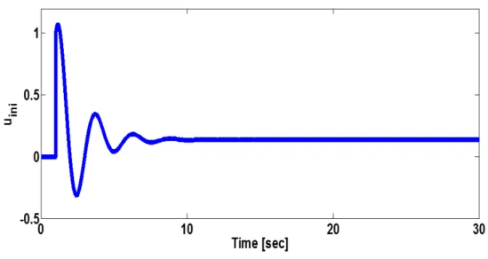
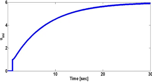
Fig. 2.3 Initial input u ini . . . . 16

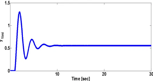
Fig. 2.4 Initial output of the inner loop y _1ini . . . . 17

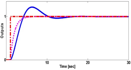
Fig. 2.5 Initial cascade control system output y _ini (solid line), reference signal r (dot-dash line), and desired output y d (dotted line). . . . 17

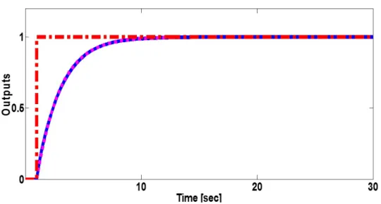
Fig. 2.6 Cascade control system output with optimal parameters y(θ ^∗ ) (solid line), the reference signal r (dot-dash line), and desired output y d (dotted line) . . . . 18

Fig. 2.7 Input with optimal parameters u(θ ^∗ ) . . . . 19

Fig. 2.8 Inner loop output with optimal parameters y ₁ (θ ^∗ ) . . . . 19

Fig. 2.9 Closed loop cascade control architecture . . . . 20

Fig. 2.10 Cascade control system outputs with optimal parameter vectors 21 Fig. 3.1 Cascade control system with tunable parameters . . . . 24

Fig. 3.2 The initial input of the inner loop. . . . 31

Fig. 3.3 Initial inner loop cascade control system output y 1ini (solid line), reference signal r (dot-dash line), and desired inner loop out- put y 1d (dotted line). . . . 32

Fig. 3.4 Inner loop cascade control system output with optimal param-

eters y ₁ (θ ^∗ )(solid line), the reference signal r (dot-dash line), and

desired inner loop output y 1d (dotted line). . . . . 33

Fig. 3.5 The input of inner loop with the optimal parameters u(θ ^∗ _II ). . . . 33

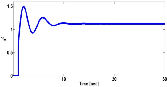
Fig. 3.6 Initial input of the outer loop cascade control system u ⁰ . . . . . 34

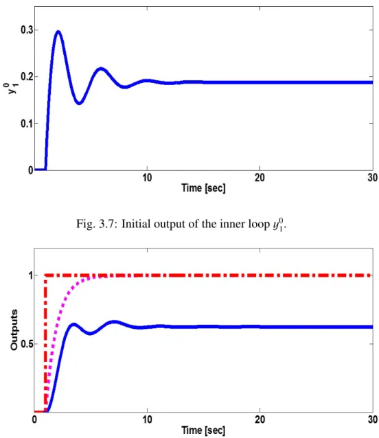
Fig. 3.7 Initial output of the inner loop y ⁰ ₁ . . . . 35

Fig. 3.8 Initial outer loop cascade control system output y ⁰ (solid line), reference signal r (dot-dash line), and desired output y d (dotted line). 35 Fig. 3.9 Cascade control system output with optimal parameters y(θ ^∗ _I ) (solid line), reference signal r (dot-dash line), and desired output y d (dotted line). . . . 37

Fig. 3.10 Input with optimal parameters u(θ ^∗ _I ). . . . 37

Fig. 3.11 Inner loop output with optimal parameters y ₁ (θ ^∗ _I ). . . . 38

Fig. 3.12 Cascade control system output with optimal parameters y(θ ^∗ _I ) (solid line) a ff ected by measurement noise, reference signal r (dot- dash line), and desired output y d (dotted line). . . . 38

Fig. 3.13 Initial outputs of outer cascade control system . . . . 40

Fig. 3.14 Cascade control system outputs with optimal parameter vectors 41 Fig. 4.1 Cascade control system with tunable parameters . . . . 44

Fig. 4.2 Initial input u ⁰ . . . . 49

Fig. 4.3 Initial output of the inner loop y ⁰ ₁ . . . . 49

Fig. 4.4 Initial cascade control system output y ⁰ (solid line), reference signal r (dot-dash line), and desired output y d (dotted line) . . . . . 50

Fig. 4.5 Cascade control system output with optimal parameters y(ρ ^∗ ) (solid line), the reference signal r (dot-dash line), and desired output y d (dotted line) . . . . 50

Fig. 4.6 Input with optimal parameters u(ρ ^∗ ) . . . . 51

Fig. 4.7 Inner loop output with optimal parameters y 1 (ρ ^∗ ) . . . . 51

Fig. 5.1 Cascade control system with tunable parameters . . . . 54

Fig. 5.2 A cascade control system with parameterized controllers θ . . . 57

Fig. 5.3 The initial input u ini . . . . 61

Fig. 5.4 The initial output of the inner loop y 1ini . . . . 62

Fig. 5.5 The initial output of cascade control system y ini (the solid line), the reference signal r (the dot-dash line), and desired output y d (the dotted line) . . . . 62 Fig. 5.6 Cascade control system outputs with optimal parameters y(θ ^∗ )

(the solid line), the reference signal r (the dot-dash line), and the desired output y d (the dotted line) . . . . 63 Fig. 5.7 Input with the optimal parameters u(θ ^∗ ) . . . . 64 Fig. 5.8 Inner loop output with the optimal parameters y ₁ (θ ^∗ ) . . . . 64 Fig. 6.1 A diagram of convention closed system with a tunable vector . 66 Fig. 6.2 A diagram of cascade control system with tunable parameters . 67 Fig. 6.3 A cascade control system with parameterized controllers ρ . . . 70 Fig. 6.4 The initial input u ini . . . . 74 Fig. 6.5 The initial output of the inner loop y _1ini . . . . 74 Fig. 6.6 The initial output of cascade control system y ini (the solid line),

the reference signal r (the dot-dash line), and desired output y d (the dotted line) . . . . 75 Fig. 6.7 Cascade control system outputs with optimal parameters y(ρ ^∗ )

(the solid line), the reference signal r (the dot-dash line), and the desired output y d (the dotted line) . . . . 75 Fig. 6.8 Input with the optimal parameters u(ρ ^∗ ) . . . . 76 Fig. 6.9 Inner loop output with the optimal parameters y ₁ (ρ ^∗ ) . . . . 77 Fig. 6.10 Cascade control system outputs with optimal parameters y(ρ ^∗ )

a ff ected by measurement noise (the solid line), the reference signal

r (the dot-dash line), and the desired output y d (the dotted line) . . . 77

Acknowledgement

Firstly, I would like to express a deep gratefulness to two academic supervi- sors, Prof. Shigeru Yamamoto and Prof. Osamu Kaneko. Especially Prof. Osamu Kaneko - from the University of Electro-Communications Chofu-Tokyo has brought me an opportunity to study on data-driven control theory to control system. Their enthusiasm, explaining, direction and encouraging words helped me so much to get successful attainment of my doctoral course in Kanazawa University.

I am also very grateful Ass. Prof. Ichiro Jikuya who supported a comfortable study environment and gave many useful advices for me in our lab.

Also many thanks to all member of MoCCoS laboratory, Mr. Phan Dinh Chung, Mr. Kengo Yamamoto for sharing knowledge. Specially Mr. Kitazaky, my tu- tor, who helped me to get on well in dealing with the documents and daily life in Kanazawa.

In addition, I want to say thank you to Vietnam International Education Devel- opment - Ministry of Education and Training (VIED) and Vietnam National Uni- versity of Agriculture which supported financially and advantageous conditions for me to pursue this research. I also want to say thank you to Dr. Nguyen Thi Hien, Dr. Nguyen Xuan Truong and Dr. Le Minh Lu, leaders of Electrical Engineering, Electrical System Departments and Faculty of Engineering -Vietnam International University of Agriculture, who gave me time and suitable advices for this PhD course. A special word or thanks sends to Dr. Nguyen Thi Hien, who introduced me to Kanzawa University and Prof. Osamu Kaneko.

I also really thank to all members of Vietnamese Student Association Kanazawa

University (Vietkindai) for helping and sharing everything in daily life in Kanazawa

city. A great regard sends to Mr. Yukio Abe, a very kind Japanese person, all Vietnamese students in Kanazawa University call him with a very respective name

”Otousan”. He always helps me and my family with the daily life matters in Kanazawa city from first day.

Above all, I would like to send thankfulness to all members of my family, par- ents, cute sons , who always encourage me for researching, and especially to my wife who spends much time to take care our children, I can be assured to concen- trate on studying.

Nguyen Quang Huy

Kanazawa, Jun 2017

Chapter 1 Introduction

1.1 Cascade control system

A cascade control system (see Fig. 1.1) is a multiple-loop system where the output of the controller in the outer loop (the “primary” or “master”) is the set point of a controller in the inner loop (the “secondary” or “slave”). The inner loop controller generates an intermediate process variable that can be used to obtain more e ff ective control of the outer process variable. Cascade control systems are developed and used for practical multiple-loop control systems, and are applied to many industrial processes such that, temperature, humidity control, pressure, level of fluids control, oil-gas industry and adjustment of DC motor speed [1, 2, 3, 4] e.g.,.

In the configuration of the cascade control system, the process is divided into two parts (the inner process and the outer process) and therefore two controllers are used, but only one signal generated from inner controller is manipulated. These two processes can be a ff ected by disturbances d 1 and d 2 , respectively.

Fig. 1.1: Block diagram of a cascade control system

The closed-loop of cascade control system can be shown in a block diagram form (Fig. 1.1). Here, the outer (master) controller generates the set point S P 2 for the inner loop which includes the inner (slave) controller and the inner process. The controlled variable of the inner loop (y ₁ ) also a ff ects the outer process and therefore it also a ff ects the primary controlled variable (y), which is also the output of cascade control system.

Cascade control system has several advantages on applications where the inner process has a large dead time or time lag . Cascade control system is also e ff ective when the large disturbance occurs in the secondary loop. Because the disturbance applied to the inner loop is eliminated by the inner controller before they a ff ect on the outer process.

The case where the cascade control system is not a ff ected by disturbances then the configuration of cascade control system can be shown in the Fig. 1.2.

Fig. 1.2: Cascade Control System

As shown in Fig.1.2, the cascade control system consists of an inner loop where an inner controller C 2 operates as a feedback controller for plant P 1 and an outer loop where an outer controller C ₁ performs the same function for inner closed loop

P

C

1 + P

C

, which is serially connected to a plant P 2 . The outer controller C 1 generates

the set point signal for the inner loop, which includes the inner controller C ₂ . The

controlled variable of the inner loop y 1 a ff ects on the outer loop y. Though this

is an ideal configuration, it is useful to analyze the mechanism of cascade control

architecture.

1.2 Data-driven Approach

Similarly to most other control architectures, appropriate mathematical models are needed to design controllers. Practically speaking, many cases exist in which a con- troller has already been designed to achieve desired specifications based on math- ematical models reflecting dynamics. It might thus be important to maintain the initial desired performance under aging changes, sudden changes, or intrinsic un- certainties. In these cases, it is desirable to develop update and tuning methods for parameters of the implemented controllers based on directly used measured data.

This is a basic principle of ” data-driven approach” to control.

Studies on data-driven controller tuning and updating have been developed such as, iterative feedback tuning (IFT, [6, 7, 8]), fictitious reference iterative tuning (FRIT, [9, 10]) and virtual reference feedback tuning (VRFT, [12, 13, 14]).

Specifically, FRIT and VRFT require only a one-shot experiment for the desir- able parameter, so they have practical advantages over IFT, which requires many experiments in o ff -line nonlinear optimization.

In the structure of cascade control system, we want to design desired controllers C 1 and C 2 , then the first important step is to obtain a mathematical model of plants P ₁ and P ₂ as exactly as possible. Controllers are designed by using conventional methods to meet a given specification based on mathematical models. Nevertheless, there are cases in where a desirable experiment to achieve mathematical model of the plants is too hard to be done. And it is also very di ffi cult to take much time and cost to execute e ffi cient experiments for identification P ₁ and P ₂ . To overcome these problems, an e ff ective solution should be used is to apply data-driven approaches to cascade control system.

In reference [5], Previdi et.al. studied VRFT design of cascade control systems

with application to an electro-hydrostatic actuator. In this work the author gave two

desired reference model (for the inner and the outer loop). The optimal parameters

of the inner controller is achieved by adjusting the inner loop to obtain tracking

properties of the inner loop so as to be approximated as desired inner reference

model with respect to the outer loop. Also, the author gave the outer desired ref-

erence model, and use the same way to find the optimal parameters of the outer controller. In fact, in the reference [5] the authors minimized the cost function and used the prefilter introduced by Campi et.al. [13] to obtain the two desired con- trollers.

As another approach of application of VRFT to cascade control systems, in my proposed method, I applied and developed VRFT methods to cascade control sys- tems in the cases in where plants are minimum and non-minimum phase systems.

Here, I construct the original cost function for cascade control system, and simul- taneously obtain optimal parameters for both inner and outer controllers by only minimizing this cost function. The most important point and di ff erent points com- pared with the Previdi’s work, I clarified the meaning of the cost function in VRFT without the prefilter. As a result, it is clarified that the cost function of VRFT aims to optimize the open loop transfer function. Moreover, I also derived the original prefilter for cascade control system not only to avoid the problem of non-properness appearing in the cost function but also to obtain the matching between optimal pa- rameters achieved from model reference criterion of VRFT and one yielded from original cost function. The above two points are major important di ff erent points compared the reference [5].

Besides, I also developed FRIT for cascade control systems in [18]. In the reference [18] , the authors have just applied FRIT method to cascade control system to deal with the case plants are minimum phases . FRIT for cascade control systems with non-minimum phase systems will be also implemented in this dissertation.

1.3 Outline of The Dissertation

The structure of dissertation consists of the following items

Chapter 2, VRFT approach to cascade control system is applied to simultane-

ously achieve the optimal parameters for both inner and outer controllers such that

the output of outer cascade control system can be approximated well with a de-

sired reference model of cascade control system. Besides, the meaning of the cost

function is also explained clearly.

Chapter 3 presents the derivation of the prefilter used in the VRFT for the cas- cade control systems, which guarantees the optimality of the cost function to be minimized. The similar method to obtain the prefilter is also used in the FRIT case, as shown in Chapter 4.

Chapters 5 and 6 presented the extensions of VRFT and FRIT for cascade con- trol systems to the non-minimum phase case. The strategy for the unstable zeros are presented.

Chapter 7 presented the concluding remarks and future works.

Chapter 2

Virtual Reference Feedback Tuning for Cascade Control Systems

Virtual Reference Feedback Tuning (VRFT), proposed by Campi et-al.,[13] is one of the e ff ective data-driven tuning methods used in feedback controllers in the sense that desired parameters implemented in the controller are obtained by using only one-shot experiment data. In this chapter, I present a VRFT method for the cascade control system. I propose a direct tuning method for controllers in cascade control system to simultaneously obtain optimal parameters for both the inner and outer controllers by performing one-shot experiment to collect a set of initial data from the cascade system. I also clarify the meaning of the cost function in my proposed method and provide an example for demonstrating our proposal’s e ff ectiveness and validity.

2.1 Cascade control systems

In the introduction part of chapter 1, cascade control system was described as multiple-loop control system ( see Fig. 1.2). It includes two loops such that inner loop and outer loop.

The inner loop the inner controller C 2 generates input control signal u to control

the plant P ₁ , and y ₁ is the output of the inner loop, it also a ff ects on the plant P ₂ of

the outer loop and the output of the cascade control system y.

The outer loop cascade contains the outer controller C ₁ operating as a feedback controller for the inner for inner closed loop ₁₊ ^P

_P ^C

1

C

, which is serially connected to a plant P ₂ . The output of the outer loop y also is the output of the cascade control system.

Consider the cascade control system with tunable parameters in Fig. 2.1.

Fig. 2.1: Cascade control system with tunable parameters

In this case, we consider that P 1 and P 2 are linear, time-invariant, single-input single-output, strictly proper, stable and minimum phase. The two controllers of cascade control system are parameterized as

C ₁ (θ) = θ n +1 q ^m + · · · + θ ν− 1 q + θ ν

q ⁿ + θ ₁ q ⁿ⁻¹ + · · · + θ _n−1 q + θ n

(2.1) and

C 2 (θ) = θ ν + n

+ 1 q ^m

+ · · · + θ µ−1 q + θ µ

q ⁿ

+ θ ν +1 q ⁿ

⁻¹ + · · · + θ ν + n

−1 q + θ ν + n

(2.2) by using a parameter vector

θ =

θ ₁ · · · θ _ν θ _{ν + 1} · · · θ _µ

. (2.3)

A transfer function with a tunable parameter vector θ from r to y is defined by T (θ), it is shown as

T (θ) = P 1 P 2 C 1 (θ)C 2 (θ)

1 + P ₁ C ₂ (θ) + P ₁ P ₂ C ₁ (θ)C ₂ (θ) (2.4) Similarly, input, output, and inner output with parameter θ are denoted by u(θ), y(θ), and y 1 (θ).

Using a parameter vector θ _ini , assume that the current or initial closed loop is

stable. The desired tracking closed loop transfer function from r to y is given as M.

The initial output y _ini : = y(θ _ini ) is di ff erent from desired output of cascade sys- tem y _d : = Mr. Here, the purpose of tuning parameters is to find optimal parameter vector θ ^∗ such that the output of cascade control system with these optimal param- eters can approximated well with the desired output y _d : = Mr.

To find the optimal parameters for both inner and outer controllers we have to minimize ky(θ ^∗ ) − Mr k ² _N and use the initial data u ini = u(θ _ini ), y _ini , and y _1ini : = y ₁ (θ _ini ).

2.2 Basic of VRFT method

In this section, I present some main points of an original VRFT method based on reference [13]. A diagram of conventional feedback system with the tunable con- troller is shown in Fig. 2.2.

Fig. 2.2: A conventional feedback control system

Here, we consider that P is a linear, time-invariant, single-input, single-output dynamical system. We also assume that P is unknown. Controller C(θ) is parame- terized by using tunable parameter vector θ : = [θ ₁ θ ₂ · · · θ _ν ] as follow:

C(θ) = θ n + 1 q ^m + · · · + θ _ν−1 q + θ _ν q ⁿ + θ ₁ q ⁿ

+ · · · + θ _n−1 q + θ n

. (2.5)

The only set of data we use is the one-shot experimental data of input u and output y. We also give desired reference transfer function M from r to y.

With above conditions, virtual reference signal ¯ r is given to satisfy

y = M r ¯ (2.6)

by using actual (initial) output, and define virtual error

¯

e : = r ¯ − y. (2.7)

Cost function

J V (θ) = ku − C(θ)¯ ek ² _N (2.8) is then minimized for θ. u is actual (initial) input and C(θ)¯ e is referred as virtual input.

Roughly speaking, the ideal minimization of J V (θ) is equivalent to that of u − C(θ)¯ e = 0, i.e., u = C(θ)¯ e = C(θ)(¯ r − Pu). The last relation is also equivalent to stating that

(1 + PC(θ)) u = C(θ)¯ r (2.9) where the right side of (2.9) is equal to

C(θ)¯ r = C(θ) 1

M y = C(θ)P

M u. (2.10)

From (2.9) and (2.10), we see that

Mu = PC(θ)

1 + PC(θ) u (2.11)

holds.

To briefly explain the mechanism of VRFT in [13], the closed loop with optimal θ is thus close to desired model M under the influence of initial input data u.

The problem of the non-properness of 1/M that appears in the virtual reference is avoided by using prefilter L = M(1 − M), which guarantees the optimality of J V

in cases where ideal minimization can not be achieved, applied to data. In [13], a more theoretical analysis of this prefilter is discussed for cases in which C(θ) is linearly parameterized, which is done by convex optimization. See [13] for details.

2.3 VRFT approach for cascade control systems

2.3.1 Construct an original cost function of cascade control sys- tems

In presenting of VRFT approach to cascade control systems, we concentrate on the inner closed loop. Applying [13] to the inner loop, we introduce cost function

J V (θ) = k u ini − C 2 (θ)¯ e 1 k ² _N . (2.12)

¯

e ₁ is the error between the initial output of inner closed-loop y _1ini and virtual refer- ence ¯ r 1 for the inner loop, which is calculated as

¯

e ₁ = r ¯ ₁ − y _1ini (2.13)

Note that ¯ r ₁ is also virtual output of outer controller C ₁ .

Now let us focus on the outer loop of the cascade control system. Similar to the inner loop, we introduce virtual error ¯ e by using actual output y _ini as follows:

¯

e = r ¯ − y _ini (2.14)

¯

r is a virtual reference such that

y _ini = M r ¯ (2.15)

for the outer loop.

As stated above, ¯ r 1 is also the output of C 1 (θ). We thus see

¯

r 1 = C 1 (θ)¯ e (2.16)

By substituting ¯ r 1 in (2.16) into (2.13) with (2.14) and (5.19), we obtain e ¯ 1 = C 1 (θ)¯ e − y 1ini

= C 1 (θ)(¯ r − y ini ) − y 1ini

= C 1 (θ) 1 M − 1

!

y _ini − y _1ini . (2.17) Last, we substitute ¯ e ₁ in (2.17) into (2.12) to obtain performance index J V (θ) of cascade control system as

J V (θ) =

u _ini + C ₂ (θ)y _1ini − C ₁ (θ)C ₂ (θ) 1 M − 1

! y _ini

2

N

(2.18) As seen trivially, J V is minimized by using only initial one-shot experimental data y ini , u ini and y 1ini . This means that our proposed method has practical advantages in cascaded controller tuning.

To minimize the above cost function J V (θ), we only perform one-shot experi-

ment on cascade control system to collect a set of initial data {u ini , y _1ini , y ini }. After

minimizing the cost function, we simultaneously obtain the optimal parameters for

both inner and outer controllers of the cascade control system such that the output of cascade control system with these optimal parameters is almost the same with desired output y d = rM. This important point is a big di ff erence from F. Previdi’s studies in [5].

In the reference [5], F. Previdi and co-authors gave a VRFT method design of cascade control systems with application to an electro-hydrostatic actuator. In the pages 628, 629 of reference [5], F. Previdi gave two desired reference models (the inner desired reference model M _v , the outer desired reference model M x ), and then he used cost functions introduced by Campi [13], J VR (θ v ) = _N ¹ P N

t = 1 (u vL (t) − C _v (θ _v )e _vL (t)) ² for the inner loop, and J VR (θ x ) = _N ¹ P N

t =1 (r _vL (t) − C x (θ x )e xL (t)) ² for the outer loop.

To obtain the tracking properties of the inner loop, he minimized the cost func- tion J VR (θ v ) to achieve the optimal parameters of the inner controller C v . Similarly, the optimal parameters of the outer controller C x are obtained by minimizing outer cost function J VR (θ x ).

From these points, we see that in my proposed method , I present an VRFT ap- proach to cascade control system such that we achieve the tracking properties of the outer cascade control system , the output of cascade control system can approximate well with desired output. Also, I calculated to establish the original cost function (equation 2.18) of VRFT method for cascade systems. Only one-shot experiment to collect the initial data is necessary for minimizing the cost function (2.18). Min- imizing this cost function simultaneously yields the optimal parameters for both inner and outer controllers. These important points are absolutely di ff erent from the study of authors in [5].

2.3.2 The meaning of the cost function with ideal case

First, we consider the meaning of J V (θ) in the ideal case, i.e., the case in which θ ^∗ exists such that J V (θ ^∗ ) = 0. In this case, note that

u ini + C 2 (θ ^∗ )y 1ini − C 1 (θ ^∗ )C 2 (θ ^∗ ) 1 M − 1

!

y ini = 0 (2.19)

holds generically. Note that trivial relations

P 1 u ini = y 1ini (2.20)

P 2 y 1ini = y ini (2.21)

Also hold. Using them, we rewrite (2.19) as 1 + P ₁ C ₂ (θ ^∗ ) − C ₁ (θ ^∗ )C ₂ (θ ^∗ )P ₁ P ₂ 1

M − 1

!!

u _ini = 0 which is equivalent to

1 + P 1 C 2 (θ ^∗ )

C ₁ (θ ^∗ )C ₂ (θ ^∗ )P ₁ P ₂ u ini = 1 M − 1

!

u ini . (2.22)

Simple algebraic manipulation of (2.22) then yields

T (θ ^∗ )u _ini = Mu _ini (2.23)

which means that the optimal closed loop is achieved over initial input.

2.3.3 The meaning of the cost function with ordinary case

It is di ffi cult to achieve J V (θ) = 0. Even in this case, we rationally interpret the minimization of J V (θ). First, note that

M

1 − M = : H M (2.24)

is interpreted as the desired open loop transfer function for M. This is because 1 − M is the sensitivity function of desired closed loop M and the open loop transfer function of the feedback loop is represented by the ratio of sensitivity function 1 − M and the complementary sensitivity function where the later function is equal to closed loop transfer function M from the reference signal to output .

Similarly, an open loop transfer function for T (θ) with parameter θ is interpreted as

T (θ)

1 − T (θ) = : H T (θ) (2.25)

From the Fig. 2.1, after some simple calculations yield H T (θ) = P ₁ P ₂ C ₁ (θ)C ₂ (θ)

1 + P 1 C 2 (θ) (2.26)

The cost function (2.18) is also rewritten as follows:

J V (θ) =

1 + P 1 C 2 (θ) − P 1 P 2 C 1 (θ)C 2 (θ) 1 M − 1

!!

u ini

2

N

=

(1 + P 1 C 2 (θ)) 1 − P 1 P 2 C 1 (θ)C 2 (θ) 1 + P ₁ C ₂ (θ)

1 H M

! u ini

2

N

=

(1 + P ₁ C ₂ (θ)) 1 − H T (θ) H M

! u _ini

2

N

(2.27) The part _{1+ P} ¹

1

C

(θ) is regarded as the sensitivity function of the inner loop.

Above equation in (2.27) shows that the minimization of J V (θ) in (2.18) corre- sponds to that of the relative error between open loop transfer function H T (θ) and H M under the influence of the inverse sensitivity function of the inner loop and initial input data u ini .

2.3.4 Algorithm

The proposed method is summarized in the following algorithm:

1. Set initial parameter vector θ _ini

2. Execute a one-shot experiment to achieve a set of data { u ini , y 1ini , y ini } . With θ _ini , controllers are assumed to stabilize the closed-loop cascade control sys- tem so that these data are bounded.

3. Calculate the virtual reference signal as r(θ) = _M ¹ y(θ ini ) and construct perfor- mance index J V (θ) as equation (2.18).

4. Minimize performance index J V (θ) using nonlinear optimization such as the Least Squares, Gauss-Newton, Gradient methods, or CMA-ES[21].

5. Obtain optimal parameter vector θ ^∗ : = arg min θ J V (θ), which yields optimal controllers and desired output of the cascade control system.

2.3.5 Remarks

To overcome the problem non-properness of _M ¹ appearing in the cost function of

VRFT to cascade control system, we have to use prefilter introduced by Campi [13],

this prefilter also guarantees the optimality of the cost function in VRFT method.

This prefilter is applied for convention system, and it can be used to avoid problem non-properness of _M ¹ in cost function (2.18). Of course, finding out an original prefilter for cascade control systems in VRFT method is an important issue which allows us to obtain better results. We will focus on this work in the next chapter.

In this method, we conducted one-shot experiment on closed loop cascade con- trol system to collect the initial data. However, we can also obtain good results in the open loop cascade control systems case.

The meaning of cost function in VRFT method for cascade control system given by equation (2.27) shows that when we minimize it, we consider the relative error between the open loop desired transfer function and the open loop transfer function cascade system. In the case of FRIT to cascade control system in [19], the meaning of the cost function is considered by the relative error between the closed loop desired transfer function and the closed loop transfer function cascade system. This point is an important di ff erence between two methods.

2.4 Numerical Example

To demonstrate the validity of the proposed method, we give an illustrative example of a cascade control system in a continuous-time domain.

Unknown plants of cascade control system are described as follows:

P ₁ = s + 8

s ² + 3s + 2 (2.28)

and

P 2 = s + 9

s ² + 7s + 5 (2.29)

The outer and inner controllers are parameterized as

C 1 (θ) = θ 1 s ² + θ 2 s + θ 3

θ ₄ s ² + θ ₅ s + θ ₆ (2.30)

and

C 2 (θ) = θ ₇ s + θ ₈ θ 9 s + θ 10

(2.31)

with θ : = [θ ₁ θ ₂ θ ₃ θ ₄ θ ₅ θ ₆ θ ₇ θ ₈ θ ₉ θ ₁₀ ] ^T .

Fig. 2.3: Initial input u _ini

The desired reference model of the cascade control systems M is given by

M = 1

s + 1 . (2.32)

Initial parameter vectors are set as

θ ini = [0.0 1.0 1.0 0.0 1.0 0.0 1.0 1.0 1.0 0.0] ^T

We then conduct a one-shot experiment on a cascade control system to obtain initial data u _ini , y _1ini and y _ini .

The initial input u ini and the initial output of the inner loop y 1ini are shown as in Fig. 2.3 and Fig. 2.4.

In Fig. 2.5, initial output of cascade control system y _ini is drawn as a solid line,

reference signal r as a dot-dash line, and desired output y d : = Mr as a dotted line.

Fig. 2.4: Initial output of the inner loop y _1ini

Fig. 2.5: Initial cascade control system output y ini (solid line), reference signal r (dot-dash line), and desired output y _d (dotted line).

By applying our proposed algorithm with VRFT and using the prefilter intro- duced by Campi [13] L = M(1 − M), the performance index J V (θ) minimization problem is solved by using covariance matrix adaptation evolution strategy CMA- ES in [21].

In this study, we programmed the CMA-ES algorithm in MATLAB and ran it

on a calculator with a 3.6 GHz Core i7-4790 CPU, 8GB RAM, and iterative step

N = 3000.

We obtained the optimal parameter vector as

θ ^∗ = [0.4664 1.7533 1.3209 0.0283 1.2162 −0.0010 0.8008 0.2504 0.0494 1.0844] ^T .

We then conducted the experiment by using optimal parameter vectors θ ^∗ , obtaining the results in Fig. 2.6.

In Fig. 2.6, the actual output of cascade control system with optimal parameter vectors y(θ ^∗ ) is shown as a solid line, reference signal r as a dot-dash line, the desired output y _d as a dotted line.

Input with optimal parameters u(θ ^∗ ) is shown in Fig. 2.7 and inner loop output with optimal parameters in Fig. 2.8.

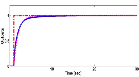
Fig. 2.6: Cascade control system output with optimal parameters y(θ ^∗ ) (solid line), the reference signal r (dot-dash line), and desired output y _d (dotted line)

Results in Fig. 2.6 show that actual output y(θ ^∗ ) and desired output y d are almost

the same, implying that we can achieve the desired output of the cascade control

system by using optimal parameter vectors θ ^∗ .

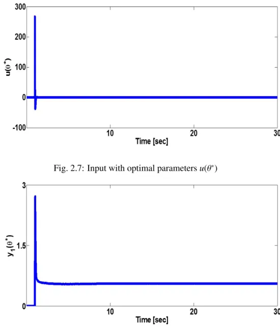
Fig. 2.7: Input with optimal parameters u(θ ^∗ )

Fig. 2.8: Inner loop output with optimal parameters y 1 (θ ^∗ )

2.5 Comparing my proposed method with F.Previdi’s method in the reference [5]

In this section, I use the method of F. Previdi in the reference [5] to apply for the same example given in the section 2.4. I also show clearly the advantage of my proposed method over than F. Previdi’s method by comparing the results of two methods.

The structure of the cascade control system which F. Previdi used in the refer-

ence [5] is given as in Fig. 2.9

Fig. 2.9: Closed loop cascade control architecture

Where the inner and outer controllers are given such as C v and C x . F. Previdi used the cost functions introduced by Campi [13] for the inner and outer loops

The cost function of the inner loop is shown such as J VR (θ _v ) =

u ⁰ − C v (θ _v ) 1 M v

− 1

! v ⁰

2

N

(2.33) And the cost function of the outer loop is

J VR (θ x ) =

r ⁰ _v − C x (θ x ) 1 M x

− 1

! x ⁰

2

N

(2.34) Where M _v and M x are desired reference models of the inner and outer loops.

The initial data { u ⁰ , v ⁰ , x ⁰ } are obtained from the cascade control system Fig. 2.9 by conducting a single experiment.

We give the desire reference model of the inner loop such as M v = _2s ¹ _{+ 1} , and choose the same desired reference model like in the section (2.4) for the outer loop such as M x = _{s +} ¹ ₁

Similarly, the structures of the inner and outer controllers are selected as

C _v (θ _v ) = θ ⁰ ₇ s + θ ⁰ ₈

θ ⁰ ₉ s + θ ⁰ ₁₀ (2.35)

and

C x (θ) = θ ⁰ ₁ s ² + θ ₂ ⁰ s + θ ₃ ⁰

θ ⁰ ₄ s ² + θ ₅ ⁰ s + θ ₆ ⁰ (2.36) Where θ _v = [θ ⁰ ₇ θ ⁰ ₈ θ ⁰ ₉ θ ₁₀ ⁰ ] ^T , θ x = [θ ₁ ⁰ θ ⁰ ₂ θ ⁰ ₃ θ ⁰ ₄ θ ⁰ ₅ θ ⁰ ₆ ] ^T

By choosing the initial data such as

θ ⁰ _v = [1.0 1.0 1.0 0.0] ^T , θ ⁰ _x = [0.0 1.0 1.0 0.0 1.0 0.0 1.0] ^T ,

we obtain the same initial output of the cascade control system as in Fig.2.5. The non-properness problems of _M ¹

and _M ¹

x

appeared in the cost functions( 2.33), (2.34) are avoided by using prefilters introduced by Campi [13] such as L _v = M _v (1 − M _v ) and L x = M x (1 − M x ).

We minimize the cost functions (2.33) and (2.34) by using a calculator with a 3.6 GHz Core i7-4790 CPU, 8GB RAM, and iterative step N = 3000 to run the CMA-ES algorithm in MATLAB.

This brings out the optimal parameter vectors for the inner and outer controllers as

θ ^∗ _v = [0.5062 0.2354 2.4708 − 0.0118] ^T

θ ^∗ _x = [0.4188 0.8970 0.7839 0.0046 1.3773 0.0061] ^T

Using these optimal parameter vectors to implement again on the cascade con- trol system Fig.2.9, we obtain the outputs of the cascade control system as in Fig.2.10

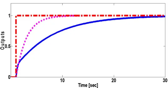
Fig. 2.10: Cascade control system outputs with optimal parameter vectors In the Fig.2.10, the solid line, dotted line and dot-dash line indicate the actual output of the cascade control system with optimal parameters, desired output and reference signal, respectively.

Obviously, when comparing result obtained by my proposed method as in the

Fig. 2.6 with the achieved result by using F. Previdi’s method as in Fig. 2.10, we see that the result in Fig. 2.10 does not satisfy the tracking property as in my result. From that observation, we can conclude that my proposed method works much better than F. Previdi’s one.

2.6 Summary

In this chapter, I presented VRFT method to the cascade control systems. Only a set data of input / output experiments collected from a closed cascade control system loop is required to simultaneously achieve the optimal parameters for both inner and outer controllers in my approach. Using optimal parameters, we are able to bring out the results showing that the output of cascade control systems is almost the same with a desired output.

Also, I have shown that VRFT method e ff ectively yields both the optimal con-

trollers in the cascade systems. Moreover, the meaning of the cost function is theo-

retically analyzed by using my proposed method.

Chapter 3

Prefilter Approach to Virtual Reference Feedback Tuning for Cascade Control Systems

In this chapter, I develop the work of chapter 2 with cascade control systems by pro- viding a more e ff ective data-driven approach. It is based on finding out an original prefilter of Virtual Reference Feedback Tuning (VRFT) method to cascade control systems.

Deriving an original prefilter of cascade control system is a very important point, it not only overcomes the problem of non-properness existed in the cost function of VRFT method but also ensures whether the optimal parameters obtained from model reference criterion in VRFT method are closed to the optimal parameters achieved from VRFT original cost function. In addition, it enables us to have a new VRFT approach to cascade control systems. Using the original prefilter is also the main di ff erence in comparison with the study by authors in reference [5].

The proposed approach allows us to obtain the optimal parameters of the in-

ner and outer controllers in the structure of cascade control systems. A numerical

example is given to demonstrate my proposal’s e ff ectiveness and validity.

3.1 Problem Formulation

Consider again a cascade control system with the tunable controller as in Fig. 3.1.

We assume that P 1 and P 2 are linear, time-invariant, single-input single-output, strictly proper, stable and minimum phase. And we also do not mention the ef- fect of the disturbance in the explanation.

Fig. 3.1: Cascade control system with tunable parameters The two controllers are parameterized as

C ₁ (θ) = θ n +1 q ^m + · · · + θ ν− 1 q + θ ν

q ⁿ + θ ₁ q ⁿ⁻¹ + · · · + θ _n−1 q + θ n

(3.1) and

C 2 (θ) = θ _{ν +} n

+ 1 q ^m

+ · · · + θ _µ−1 q + θ _µ q ⁿ

+ θ ν + 1 q ⁿ

^{− 1} + · · · + θ ν + n

−1 q + θ ν + n

(3.2) by using a parameter vector

θ =

θ ₁ · · · θ ν θ ν +1 · · · θ µ

. (3.3)

A transfer function with a tunable parameter vector θ from r to y is denoted by G ry (θ), which is represented as

G ry (θ) = P 1 P 2 C 1 (θ)C 2 (θ)

1 + P ₁ C ₂ (θ) + P ₁ P ₂ C ₁ (θ)C ₂ (θ) (3.4) Similarly, input, output, and inner output of cascade system with parameter θ are denoted by u(θ), y(θ), and y 1 (θ).

Using a parameter vector θ ⁰ , we assume that with this parameter the initial out- put of the closed loop cascade control system is bounded.

The desired reference model of a closed loop cascade system is given by M.

Initial output y ⁰ : = y(θ ⁰ ) is di ff erent from the desired output y d : = Mr. Here, the

optimal parameter vector θ ^∗ is found by minimizing ky(θ ^∗ ) − Mrk ² _N and using the

initial data u ⁰ : = u(θ ⁰ ), y ⁰ , and y ⁰ ₁ : = y 1 (θ ⁰ ).

3.2 Prefilter for Virtual Reference Feedback Tuning in the structure of cascade control systems

3.2.1 VRFT approach to cascade control systems

Standard of VRFT method for a convention closed-loop control system (Fig. 2.2) is shown by M. Campi [13]. It is based on minimizing the criterion index to obtain the optimal parameters for the controller.

J _VR ^N (θ) = 1 N

N

X

t = 1

[u(t) − C(θ)e(t)] ² (3.5)

In the chapter 2, I have applied VRFT method to cascade control systems. As shown in the chapter 2 and reference [27], a virtual reference signal ¯ r of cascade control system is introduced to satisfy

y = M r ¯ (3.6)

And the criterion index of cascade control system J _VR ^K (θ) is described as J _VR ^K (θ) = 1

K

K

X

t = 1

"

u(t) + C ₂ (θ)y ₁ (t) − C ₁ (θ)C ₂ (θ) 1 M − 1

! y(t)

# 2

(3.7) In here, we note that the output of the inner loop y ₁ (t) and the output of the outer loop cascade control y(t) are expressed through the input u(t) such that

y ₁ (t) = u(t)P ₁ and y(t) = y ₁ (t)P ₂ = u(t)P ₁ P ₂

Hence, the criterion index of cascade control system J _VR ^K (θ) can be described as J _VR ^K (θ) = 1

K

K

X

t = 1

"

1 + C 2 (θ)P 1 − C 1 (θ)C 2 (θ)P 1 P 2

1 M − 1

!!

u(t)

# 2

(3.8) By using a compatible prefilter L c , the signals u(t), y ₁ (t) and y(t) are filtered into L c u(t), L c y 1 (t) and L c y(t), respectively.

When the number of data increases (K → ∞), using the discrete Parseval theo- rem [28, 29], the criterion J _VR ^K (θ) is rewritten in the frequency domain as

J VR (θ) = 1 2π

Z π

−π

L c

"

1 + C 2 (θ)P 1 − C 1 (θ)C 2 (θ)P 1 P 2

1 M − 1

!#

2

Φ ^u dω (3.9)

Where Φ ^u is the power spectrum density of u(t).

3.2.2 Derivation of original prefilter for cascade control systems

As stated above, the purpose of control in VRFT approach to cascade control system scheme is to achieve the optimal parameter vector θ ^∗ by minimizing the following model reference criterion

J MR (θ) =

G ry (θ) − M

2 2

=

P 1 P 2 C 1 (θ)C 2 (θ)

1 + P ₁ C ₂ (θ) + P ₁ P ₂ C ₁ (θ)C ₂ (θ) − M

2 N

(3.10) With a reference signal r is used as a virtual input of the cascade control system, we expect that it yields the desired output of cascade system.

Model reference criterion of cascade control system J MR (θ) can be described as J _MR ^N (θ) = 1

N

N

X

t =1

h Mr − G _ry (θ)r i 2

(3.11) Similarly to section 3.1, when N → ∞ using the discrete Parseval theorem [28, 29]

we obtain

J MR (θ) = 1 2π

Z π

−π

G _ry (θ) − M

2 Φ r dω (3.12)

Where Φ r is the power spectrum density of the signal r.

We introduce two ideal controllers C ^d ₁ and C ₂ ^d such that P ₁ P ₂ C ₁ ^d C ^d ₂

1 + P 2 C ^d ₂ + P 1 P 2 C ^d ₁ C ₂ ^d = M (3.13) In the scheme of cascade control system, C ^d ₁ , C ^d ₂ are chosen to satisfy the problem model-matching such that the output of closed loop cascade control system is equal to the desired output Mr.

By substituting the desired reference model of the cascade control system M in (3.13) to equation (3.12), and after some simple calculations, the model reference criterion J MR (θ) is rewritten as

J MR (θ) = 1 2π

Z π

−π

P 1 P 2 C 1 C 2

1 + P ₁ C ₂ + P ₁ P ₂ C ₁ C ₂ − P ₁ P ₂ C ^d ₁ C ₂ ^d 1 + P ₁ C ₂ ^d + P ₁ P ₂ C ₁ ^d C ^d ₂

2

Φ r dω

= 1 2π

Z π

−π

| P 1 P 2 | ² | C 1 C 2 (1 + P 1 C ^d ₂ ) − C ^d ₁ C ₂ ^d (1 + P 1 C 2 ) | ²

|1 + P ₁ C ₂ + P ₁ P ₂ C ₁ C ₂ | ² |1 + P ₁ C ^d ₂ + P ₁ P ₂ C ^d ₁ C ₂ ^d | ² Φ ^r dω (3.14)

We consider again the cost function J VR (θ) in (3.9) used in the VRFT framework for cascade control system. By using prefilter L c and substituting M in (3.13) to equation (3.9) and after some calculations, we obtain the representation for cost function J VR (θ) of cascade control system as follows

J VR (θ) = 1 2π

Z π

−π

|L c | ² |P ₁ P ₂ | ² |C ₁ C ₂ (1 + P ₁ C ^d ₂ ) − C ^d ₁ C ^d ₂ (1 + P ₁ C ₂ )| ²

| M | ² |1 + P 1 C ^d ₂ + P 1 P 2 C ^d ₁ C ^d ₂ | ² Φ u dω (3.15) By comparing equation (3.14) with equation (3.15), the prefilter L c is chosen as

|L c | ² = |M| ²

|1 + P 1 C 2 + P 1 P 2 C 1 C 2 | ² Φ r

Φ ^u (3.16)

to guarantee that J VR (θ) = J MR (θ) and hence minimizing J VR (θ) is the same as minimizing J MR (θ).

In addition, from the equation (3.13) we acquire 1

|1 + P ₁ C ^d ₂ + P ₁ P ₂ C ^d ₁ C ₂ ^d | ² = |1 − M| ²

|1 + P ₁ C ₂ ^d | ² (3.17) In here, the purpose of control is to obtain the model-matching problem such as the output of cascade control system equals to the desired reference model output y = Mr. So, we expect that |1 + P ₁ C ₂ + P ₁ P ₂ C ₁ C ₂ | ² ≈ |1 + P ₁ C ^d ₂ + P ₁ P ₂ C ^d ₁ C ^d ₂ | ² and

| 1 + P 1 C 2 | ² ≈ | 1 + P 1 C ₂ ^d | ² for

argminJ MR (θ) = argminJ VR (θ) (3.18)

With above respect, the prefilter L c need to satisfy

| L c | ² = | M | ² |1 − M | ² 1

|1 + P 1 C 2 | ² Φ r

Φ ^u (3.19)

In the equation (3.19), the prefilter L c is still unclear since the term _{|1 + P} ¹

1

C

|

remains unknown. However, we can overcome this di ffi culty by a strategy given in the next explanation.

In the diagram of cascade control system Fig. 3.1, we concentrate on the inner loop where the sensitivity function of the inner loop is given by

S i = 1 − P 1 C 2

1 + P ₁ C ₂ = 1

1 + P ₁ C ₂ (3.20)

If M ₁ is a desired reference model of the inner loop, we expect that it is possible to obtain the model-matching of the inner loop such that the closed loop transfer function of the inner loop is equal to the desired reference model M ₁

P 1 C 2

1 + P ₁ C ₂ = M 1 (3.21)

If we hold the above condition, then the sensitivity function of the inner loop S i is rewritten as

S i = 1

1 + P ₁ C ₂ = 1 − M 1 (3.22)

Finally, we obtain the original prefilter L c of the cascade control systems by substituting equation (3.22) to equation (3.19) to get

|L c | ² = |M| ² |1 − M| ² |1 − M ₁ | ² Φ ^r Φ u

(3.23) The derivation of above original prefilter L c enables us to have a new strategy in applying VRFT approach to cascade control systems. This is an important di ff erent point from the work of the chapter 2 and [27].

Besides, finding out the original prefilter of VRFT method for cascade control system in equation (3.23) is also the main di ff erence in comparison with work of F.

Previdi and co-authors in [5]. In the pages 628, 629 of the reference [5], F. Previdi only used the cost function and prefilter introduced by Campi [13] for using VRFT method to apply to an electro-hydrostatic actuator.

By constructing the cost function of outer loop cascade system as equation (2.18) with original prifilter of cascade system in (3.23), we can achieve the track- ing properties problem of cascade control system such that the output of cascade control system y(θ ^∗ ) with optimal parameters can be almost the same with desired output y d = rM.

Identify prefilter L c :

The original prefilter of cascade control system L c in (3.23) can be calculated

exactly if we know the power spectrum density of r, u signals as Φ r , Φ u . In this

case, before implementing an experiment on structure of cascade control system,

the designer should decide the kind of excited input signal and author also should

consider to estimate Φ ^r and Φ ^u .

In another case, the original prefilter of cascade control system L c can be con- sidered to identify as follows:

From equation (3.23), under the e ff ect of the initial signals r ⁰ , u ⁰ , the original prefilter of cascade systems can be selected as

L c u ⁰ = M(1 − M)(1 − M ₁ )r ⁰ (3.24) If we give a structure of the original prefilter L c and parameterize it by vector η = [η ₁ η ₂ ... η n ] ^T , then we establish the cost function of L c as

J L

(η) = k L c (η)u ⁰ − M(1 − M)(1 − M 1 )r ⁰ k ² _N (3.25) Where the initial data r ⁰ , u ⁰ are collected from cascade control system by one-shot experiment, M ₁ and M are desired reference models of the inner loop and outer loop.

The optimal parameters of the original prefilter cascade control system L c can be obtained by minimizing the cost function (3.25) as

η ^∗ = argmin _η J L

(η) (3.26)

3.2.3 Algorithm

We summarize the proposed method by the following algorithm:

In the scheme of cascade control system Fig. 3.1 we implement

1. Tuning inner loop of the cascade control system to obtain the optimal inner controller C 2 (θ ^∗ _II ):

• Given a reference model M ₁ of the inner loop cascade control systems

• As presented in [13], we construct the cost function of the inner loop such as

J VR

(θ II ) =

u ini − C ₂ (θ II ) 1 M ₁ − 1

! y _1ini

2

N

(3.27)

Where: {u ini , y _1ini } are initial data of the inner loop. We also can use prefilter of Campi in [13] L 1 = M 1 (1 − M 1 ) to avoid the problem of the non-properness of _M ¹

1

that appears in the above cost function.

• Minimizing the cost function (3.27) to achieve the optimal parameters of the inner controller C ₂ (θ ^∗ _II ).

2. Tuning outer loop of cascade control system, which includes the outer con- troller C 1 (θ I ) and the optimal inner controller C 2 (θ ^∗ _II ) to achieve the optimal outer controller C ₁ (θ ^∗ _I ) :

• A desired reference model of the outer loop cascade control system is given by M. Conducting the second experiment on outer cascade con- trol systems to obtain a set of initial data {u ⁰ , y ⁰ ₁ , y ⁰ } from cascade con- trol system. With these initial data, the outer controller is assumed to stabilize the closed-loop cascade control system so that these data are bounded.

• As shown in the chapter 2 and reference [27], using the original prefilter L c derived in the equation (3.23), the cost function of the outer loop cascade control system is described as

J VR

(θ I ) =

L c u ⁰ + C ₂ (θ ^∗ _II )L c y ⁰ ₁ − C ₁ (θ I )C ₂ (θ ^∗ _II ) 1 M − 1

! L c y ⁰

2

N

(3.28)

• Minimize the cost function (3.28) using nonlinear optimization methods such as the Least Squares, Gauss-Newton, Gradient methods, or CMA- ES [21] to obtain the optimal parameters of outer controller C ₁ (θ ^∗ _I ).

3.3 Numerical Example

In this section we demonstrate the validity of the proposed method by giving an

illustrative example of a cascade control system in a continuous-time domain and

assume that it is not a ff ected by disturbance.

Two unknown plants of cascade control system are described as follows:

P ₁ = s + 1

s ² + 5s + 6 (3.29)

and

P ₂ = s + 5

s ² + 2.5s + 1.5 (3.30)

Firstly, we will turn the closed- loop inner of cascade control system to guarantee that the sensitivity function of the inner loop is approximate to the desired reference model of the inner loop M ₁ .

A desired reference model of the inner loop is given by:

M 1 = 1

2s + 1 (3.31)

The inner controller is parameterized as:

C ₂ (θ II ) = θ 1 s ² + θ 2 s + θ 3

θ ₄ s ² + θ ₅ s + θ ₆ (3.32)

with θ II : = [θ ₁ θ ₂ θ ₃ θ ₄ θ ₅ θ ₆ ] ^T .

We use an initial parameter vector θ _IIini = [0.0 1.0 1.0 0.0 1.0 0.0] ^T , and then conduct an one-shot experiment on the inner closed-loop cascade control system to obtain initial data {u _ini , y _1ini }. The initial input of the inner loop is shown in Fig. 3.2.

Fig. 3.2: The initial input of the inner loop.

Fig. 3.3: Initial inner loop cascade control system output y _1ini (solid line), reference signal r (dot-dash line), and desired inner loop output y 1d (dotted line).

In Fig. 3.3, the initial output of the inner loop cascade control system y _1ini is the solid line, reference signal r is the dot-dash line and the desired inner loop output y _1d : = M ₁ r is the dotted line.

We can obtain the cost function of the inner loop by using equation (3.27) and the prefilter introduced by Campi [13] L ₁ = M ₁ (1 − M ₁ ). Then the cost function J VR

(θ II ) minimization problem is solved by using covariance matrix adaptation evolution strategy CMA-ES in [21].

Here, a calculator with a 3.6 GHz Core i7-4790 CPU, 8GB RAM, and iterative step N = 1000 are used to run CMA-ES algorithm program in MATLAB.

The optimal parameter vector of the inner controller is achieved as θ ^∗ _II = [0.3338 1.3079 1.5522 0.5180 0.5176 0.0] ^T .

We implement the experiment again on the inner loop cascade control system by using the optimal parameter vector θ ^∗ _II to obtain the results in Fig. 3.4, in this figure the actual output of the inner loop cascade control system with optimal parameter vector y ₁ (θ ^∗ _II ), the reference signal r and the inner desired output y _1d are shown in solid line, dot-dash line and dotted line respectively.

We also achieve the input of the inner loop with the optimal parameters u(θ ^∗ _II )

as in Fig. 3.5.