Partial Differential Equation Approach and Convolutional Neural Network Approach to Image Processing and Its Application

Convolutional Neural Network Approach to Image Processing and Its Application

著者 モハマド ハフィズ

著者別表示 Mochammad Hafiizh journal or

publication title

博士論文要旨Abstract 学位授与番号 13301甲第5005号

学位名 博士（理学）

学位授与年月日 2019‑09‑26

URL http://hdl.handle.net/2297/00056473

Creative Commons : 表示 ‑ 非営利 ‑ 改変禁止 http://creativecommons.org/licenses/by‑nc‑nd/3.0/deed.ja

Partial Differential Equation Approach and Convolutional Neural Network Approach to Image Processing and Its

Application

Graduate School of

Natural Science & Technology Kanazawa University

Division of Mathematical and Physical Science

Student ID No. 1624012013

Name Mochammad Hafiizh

Chief Advisor Prof. Seiro Omata

28 June 2019

This study is about two approaches to image processing. The first approach is the partial differential equation. This consists of the active contour method, the curvature of the outer edge, and the Fourier transformation. From the Fourier transformation, we consider the frequency and the magnitude. The results show that if the zero frequency is the maximizer of the magnitude, then the capillary is straight. Otherwise, the capillary is wiggly. The second approach is the convolutional neural network. The training dataset to update the parameters of the model consists of the labeled hand-drawn image of each category. We use transfer learning, VGG16-model, and modify some layers near the end. The results show that this second approach is successfully classified the capillaries into two categories. However, there are a few cases which both approaches classified the capillary incorrectly.

Dissertation Abstract

1 Introduction

Image processing has some interesting topic to be discussed academically, for example, image segmen- tation, classification, recognition, reconstruction, etc. Among all of those, the classification problem is chosen in this study. Two different approaches to classify the images are proposed. Those approaches are the partial differential equation and the convo-

lutional neural network.

_{Figure 1:} The image of

capillaries taken by a micro- scope.

Those approaches are applied to the image of the capillary in human fingertips. The

capillaries of human fingertips could give important information about the healthiness

[6], [5]. However, the aim of this study is to classify the capillaries into two categories,

that are wiggly and straight. The straight capillary means its shape goes relatively

straight toward the tip of a finger. Then it turns back forming much less a half of ellipse

or circle, let say this is a turning point. Finally, it goes relatively straight, parallel to the

first move before it turns, see Figure 1. Otherwise, that capillary is defined as a wiggly

capillary.

2 Partial Differential Equation Approach

2.1 Active contour method

Let f : Ω

→R

be a given image, where Ω

⊂R²

is an open set. Let the initial contour be the zero level set of the given function φ

₀

: Ω

→ R. Let

φ : [0,

∞)×

Ω

→ R

where φ(0, x, y) = φ

₀

(x, y). The evolution of φ have to satisfy:











∂φ

∂t

= δ(φ)

h

−λ₁|f−

c

₀|²

+ λ

₂|f−

c

₁|²

+ γ div

_∇φ

|∇φ|

i

, in (0,

∞)×

Ω φ = φ

0

, in

{0} ×

Ω

δ(φ)

|∇φ|

∂φ

∂n

= 0, on (0,

∞)×

∂Ω.

(1)

where λ

₁

, λ

₂

, γ are the positive fixed constants, δ is the delta dirac function, c

₀

is the average of f in the interior of the zero level set of φ, c

1

is the average of f in the exterior of the zero level set of φ , and

^∂φ_∂n

denotes normal derivative of φ at the boundary. The delta dirac function is approximated by δ

= H

⁰

where H

(x) =

¹₂

1 +

²_π

arctan

^x

. [3] said that the zero level set of φ evolves toward the edge of an object on f .

2.2 Curvature

We show brief explanation about curvature here. For more details, see [4]. Let a curve C : (0, 1)

→

Ω be given. Let ζ(t) = (x(t), y(t)) where t

∈

(0, 1) be the parametric representation of C, where x, y : (0, 1)

→ R

and both x and y are twice continuously differentiable and (x

⁰

(t))

²

+ (y

⁰

(t))

² 6= 0,∀t∈

(0, 1) . Let the curvature be k : (0, 1)

→R,

then it could be calculated as

k(t) = x

⁰⁰

(t)y

⁰

(t)

−

y

⁰⁰

(t)x

⁰

(t)

(x

⁰

(t))

²

+ (y

⁰

(t))

²

³₂

(2) where t

∈

(0, 1).

2.3 Fourier Transformation

For more details explanation, see [1]. Let η : (0, 1)

→R, then the Fourier Transformation

of η , denoted by η ¯ , is defined by

¯ η(k) =

Z 1 0

η(x)e

^−2πikx

dx, (3)

where k is called the frequency. The magnitude is defined by

|¯

η(k)| . There are some

properties which are quite useful. First, the magnitude is an even function. Second, if

η > 0, then the peak magnitude occurs at the zero frequency. The same results happen when η < 0 .

3 Convolutional Neural Network Approach

This chapter explains briefly about the convolu- tional neural network, for more details, see [2].

Mathematically, one could describe a neural net- work as a mapping from a set of inputs to a set of output which is determined by the parameters that could be adjusted. One could see it as the process of a set of inputs that pass through one or more layers, where in each layer there is a set of nodes, before producing a set of outputs. Figure 2 shows an example of a model of fully connected neural networks with N -layers.

Input Layer-1

...

Layer-2

...

. . .Layer-n

...

. . .Layer-N

... Ouput

Figure 2: A sample of N-layers neural networks.

The circle or node indicates the perceptron.

The ideas of the convolutional neural network are local receptive area, the sharing weight, and sub-sampling. The local receptive area would keep the spatial domain of the input.

The sharing weight affects the number of parameters is much reduced. The sub-sampling affects whenever the input image is translated, the activations of the feature map would be translated by the same amount, but the other feature maps would be not changed.

Let the input be x = ((x

_ij

))

∈M^m1×m2

, an image of the size (m

₁

, m

₂

), and the activation function f

c

be defined component-wise. For example, if z = ((z

ij

))

∈ M^mz1×mz2

, then f

c

(z) = ((f (z

ij

)))

∈ M^mz1×mz2

where f :

R → R. An example of the activation

function is tanh(·) or max(0,

·). Then the output of node-q

at first layer, indicated by the superscript (1), is

y

⁽¹⁾_q

= f

_c⁽¹⁾

w

⁽¹⁾_q ∗

x + w

⁽¹⁾_0q

, (4)

where q = 1, 2, 3, . . . , Q

⁽¹⁾

, the output y

_q⁽¹⁾ ∈ M^q

(1)

1 ×q₂⁽¹⁾

for some q

⁽¹⁾₁ ≤

m

₁

, q

⁽¹⁾₂ ≤

m

₂

, the weight or known by the kernel is w

q⁽¹⁾ ∈ M^m

(1)

q1×m⁽¹⁾_q2

, the bias is w

⁽¹⁾_0q ∈ M^q

(1) 1 ×q₂⁽¹⁾

, and the component-wise activation is f

c⁽¹⁾

. For the layer-n, the output of node-q is

y

⁽ⁿ⁾_q

= f

_c⁽ⁿ⁾





Q⁽ⁿ⁻¹⁾

X

p=1

w

⁽ⁿ⁾_q ∗

y

⁽ⁿ⁻¹⁾_p

+ w

⁽ⁿ⁾_0q





, (5)

where n = 2, 3, 4, . . . , N, q = 1, 2, 3, . . . , Q

⁽ⁿ⁾

, the output y

q⁽ⁿ⁾ ∈ M^q

(n)

1 ×q⁽ⁿ⁾₂

for some q

₁⁽ⁿ⁾ ≤

q

₁⁽ⁿ⁻¹⁾

, q

₂⁽ⁿ⁾≤

q

₂⁽ⁿ⁻¹⁾

, the weight or known by the kernel is w

⁽ⁿ⁾q ∈ M^m

(n) q1 ×m⁽ⁿ⁾_q2

, the bias is w

⁽ⁿ⁾_0q ∈M^q

(n)

1 ×q⁽ⁿ⁾₂

, and the component-wise activation is f

c⁽ⁿ⁾

. Once we have

the output, then the losses function is defined to measure how close the output to the

targeted output. The task now is to find the optimum parameters such that the losses

function is as low as possible. This could be done by using the gradient descent method.

The process of updating the parameters is called training.

Transfer learning means that we transfer the model and its optimum parameters from the other results after it is trained on a huge amount of training dataset. Then at the end of that model, it is added the desired layers or classifiers. That model is a so-called pre-trained model. In this study, VGG16 is used as the pre-trained model.

4 Application

Figure 3: The evolution of the given curve (red) on the given three different images.

0 5 10 15 20

0.000 0.005 0.010 0.015

0 5 10 15 20

0.000 0.005 0.010 0.015

0 5 10 15 20

0.000 0.005 0.010 0.015

0.0 0.2 0.4 0.6 0.8 1.0

0.4 0.2 0.0 0.2 0.4

0.0 0.2 0.4 0.6 0.8 1.0

0.4 0.2 0.0 0.2 0.4

0.0 0.2 0.4 0.6 0.8 1.0

0.4 0.2 0.0 0.2 0.4

0 5 10 15 20

0.000 0.002 0.004 0.006 0.008

0 5 10 15 20

0.000 0.002 0.004 0.006 0.008

0 5 10 15 20

0.000 0.002 0.004 0.006 0.008

0.0 0.2 0.4 0.6 0.8 1.0

0.02 0.01 0.00 0.01 0.02

0.0 0.2 0.4 0.6 0.8 1.0

0.02 0.01 0.00 0.01 0.02

0.0 0.2 0.4 0.6 0.8 1.0

0.02 0.01 0.00 0.01 0.02

0 5 10 15 20

0.000 0.005 0.010 0.015 0.020

0 5 10 15 20

0.000 0.005 0.010 0.015 0.020

0 5 10 15 20

0.000 0.005 0.010 0.015 0.020

0.0 0.2 0.4 0.6 0.8 1.0

0.4 0.2 0.0 0.2 0.4

0.0 0.2 0.4 0.6 0.8 1.0

0.4 0.2 0.0 0.2 0.4

0.0 0.2 0.4 0.6 0.8 1.0

0.4 0.2 0.0 0.2 0.4

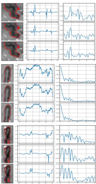
Figure 4: The longest outer curve (left), its curvature (middle), and its magnitude of

Fourier transformation (right).

Applying (1) for f as the image of capillary gives quite good results when detecting the

edge of the capillary, see Figure 3. The longest outer edge is then chosen. Its curvature

is measured by 2. Then the magnitude of its Fourier transformation is calculated. Let consider the first six rows in Figure 4. It could be seen in the middle column that the curvature for the wiggly capillary oscillates significantly. Although there are oscillations in the curvature of the straight capillary, but the hill is quite dominant. Therefore, the peak magnitude of the Fourier transform occurs at zero frequency. For the wiggly capillary, the peak magnitude occurs at the nonzero frequency, close to 4. This result is successfully used to classify the capillary into wiggly or straight. However, the last three rows in Figure 4 shows the straight capillary has a jump and the melted edge near the turning point. The zero frequency is not the maximizer of the magnitude of the Fourier transformation. Then for this case, this first approach incorrectly classifies this capillary into the straight.

The second approach is the convolutional neural net- work which in this study is implemented in Python and Torch. First, the pre-trained model VGG16 and its parameters were downloaded. Its end-layer then modified such that the output would be the score for each category, that is straight and wiggly capillary.

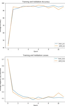
The hand-drawn images for the training, validation, and test dataset are created. It is then generated more by stretching or shrinking, rotating by small angles, and adding a noise such that there are 360 im- ages for the training dataset and 180 images for each validation and test dataset. The training dataset is used to update the parameters of the model while the validation dataset is used to see the performance of the updating process. Figure 5 shows the losses func- tion and accuracy during the updating process. After 11 epochs, the training is stopped since the accuracy and the losses are relatively stable at higher than 90% and 0.2 respectively. The parameters that are obtained at epoch 11 are chosen to be the optimum parameters. When it is used on the test dataset, the accuracy is 97%. This means out of 180 images, only 5 images are incorrectly classified.

Figure 5: The result of the pro- cess of the updating parameters of

the model.

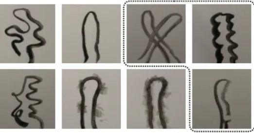
Next, the model is applied to the second test dataset, see Figure 6. It consists of the hand-drawn images but it is not created by the author. This second test dataset is generated without prior knowledge about the images on the training, the validation, and the first test dataset. By labeling the first column of as the wiggly and the rest is a straight, the accuracy of the model is 62.5%. This second approach incorrectly classifies the straight capillary when there is a jump, cross-section, or the changing curvature often.

Figure 6: The second test dataset. The three images blocked by the dotted line are classified in-

correctly.

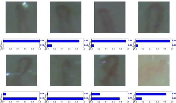
Last, the test dataset is the images of capillaries taken by a microscope. Our naked eyes could decide clearly that the capillary in the first row of Figure 7 is straight. By looking at the score below each image, this second approach successfully classifies these images. However, the third row of Figure 7 shows the capillaries which our naked eyes are difficult to label it. Hence, we consider the score of each image on each category.

Let consider the third row of Figure 7 from left to the right. The left image seems the straight capillary but there is a little curve. The convolutional neural network gives score for the wiggly quite higher, 0.92. The second image also seems straight but it is not quite clear to be seen by naked eyes. Unfortunately, by looking at the blue bar below ths image, this second approach classifies this capillary as the wiggly. There is self cross-section in the third image. The score of wiggly category is 0.77, higher than the score for the straight. This is as the expectation. Although the right image could not clearly be seen, it seems a wiggly capillary. However, this second approach classified it as the straight.

5 Conclusion

The partial differential equation approach and the convolutional neural network ap- proach works well on the classification of the image of the capillaries in human fingertips.

For the first approach, the results show that it could be almost the perfect classifier.

Detecting the outer edge is done by the active contour method. This method works well even for the noisy image. From the outer edge, the curvature is approximated. It then transformed by Fourier. The results show that the straight capillaries have zero frequency as the maximizer of the magnitude. The wiggly capillaries have a nonzero frequency at which the peak magnitude occurs.

The advantage of this first approach is that it could be implemented directly to the image

independently. Even if the image is a little noisy, it still works. How much the curvature

bend could also be detected by this method. The disadvantage of this approach is that

it does not work well when there is a jump, cross section, or melted edge of a straight

0.0 0.2 0.4 0.6 0.8 1.0 wiggly

straight 0.00

1.00

0.0 0.2 0.4 0.6 0.8 1.0

wiggly

straight 0.13

0.87

0.0 0.2 0.4 0.6 0.8 1.0

wiggly

straight 0.06

0.94

0.0 0.2 0.4 0.6 0.8 1.0

wiggly

straight 0.06

0.94

0.0 0.2 0.4 0.6 0.8 1.0

wiggly

straight 0.92

0.08

0.0 0.2 0.4 0.6 0.8 1.0

wiggly

straight 0.98

0.02

0.0 0.2 0.4 0.6 0.8 1.0

wiggly

straight 0.77

0.23

0.0 0.2 0.4 0.6 0.8 1.0

wiggly

straight 0.16

0.84

Figure 7: The results of the model when it is applied to the images of capillary taken by a microscope.

capillary. Another lack is that it is relatively not easy to determine the appropriate distance between three points which are used to calculate the curvature. If this distance is too close, the noise effect could affect the curvature quite high positively or negatively.

If the distance is too far, the important information of the curvature would be lost.

The second approach is the convolutional neural network. This second approach is able to classify the image of the capillary quite well. From the first test dataset which almost similar to the training dataset, 97% of 180 images are classified correctly. When it is applied to the second test dataset which is completely different than the first, not generated by the author, and a representation of some possibility that might happen to the capillary, out of 8 images, its accuracy is 62.5%. For the image taken by a microscope, labeling by the naked eyes whether it is straight or wiggly is not an easy task. However, some images are able hardly to be labeled. When we forced to give a label, then 71.4% of 7 images are classified correctly.

The disadvantage of this approach is that it needs a huge amount of dataset on the training. The computational cost to obtain the optimum parameters is high. The more images used in the training dataset, the better the performance of the model and the more time is needed to train. This model does not work well on the image of a straight capillary which has a jump, cross section, or changed curvature often. However, this last lack could happen because there is no image similar to these case in the training dataset.

The advantage of this approach is that once the optimum parameters are obtained, the

computational cost in the test dataset is quite fast. Even in the melted edge of the

capillary, this model works well.

Bibliography

[1] Bailey, D. and Swarztrauber, P. (1994). A Fast Method for the Numerical Eval- uation of Continuous Fourier and Laplace Transforms. SIAM Journal on Scientific Computing, 15(5):1105–1110.

[2] Bishop, C. M. (2006). Pattern recognition and machine learning. Information science and statistics. Springer, New York.

[3] Chan, T. F. and Vese, L. A. (2001). Active contours without edges. IEEE Transac- tions on Image Processing, 10(2):266–277.

[4] Goldman, R. (2005). Curvature formulas for implicit curves and surfaces, volume 22.

Computer Aided Geometric Design.

[5] Hung, C. N. D., Ito, T., and Hashimoto, I. (2012). Classification of capillary im- ages based on the average curvature estimation. The Science Report of Kanazawa University, (56):35–44.

[6] Ogawa, S. (1994). Mousaikekkanzou to Rinnshou. Toriumi Shobo.

9