Data Preprocessing for Improving Cluster Analysis and Its Application to Short Text Data

Analysis and Its Application to Short Text Data

著者 チャン ブゥ アン

著者別表示 Tran Vu Anh journal or

publication title

博士論文本文Full 学位授与番号 13301甲第4317号

学位名 博士（工学）

学位授与年月日 2015‑09‑28

URL http://hdl.handle.net/2297/43864

doi: 10.4236/jsea.2014.78059

Creative Commons : 表示 ‑ 非営利 ‑ 改変禁止 http://creativecommons.org/licenses/by‑nc‑nd/3.0/deed.ja

i

Data Preprocessing for Improving Cluster Analysis and Its Application to Short Text Data

Graduate School of

Natural Science & Technology Kanazawa University

Division of Electrical Engineering and Computer Science

Student ID No.: 1223112012 Name: Tran Vu Anh

Chief advisor: Professor Kenji Satou

Date of Submission: July 3 ^rd , 2015

ii

Table of contents

CHAPTER I Dissertation introduction ... 1

1.1 Dissertation overview ... 1

1.2 Dissertation distribution ... 2

CHAPTER II Clustering and data preprocessing for clustering ... 3

2.1 Clustering ... 3

2.1.1 Background of clustering ... 3

2.1.2 Challenges in clustering ... 4

2.2 Data preprocessing ... 5

CHAPTER III Data preprocessing algorithm D-IMPACT ... 7

3.1 Gravity-based data preprocessing algorithm ... 7

3.2 Clustering algorithm IMPACT ... 8

3.2.1 IMPACT algorithm ... 8

3.2.2 Experiment result ... 15

3.3 Data preprocessing algorithm D-IMPACT ... 19

3.3.1 Movement of data points ... 20

3.3.1.1 Density ... 20

3.3.1.2 Attraction ... 21

3.3.1.3 Inertia value ... 22

3.3.1.4 Data point movement ... 22

3.3.2 D-IMPACT algorithm ... 23

3.3.2.1 Noisy points and outlier detection ... 24

3.3.2.2 Moving data points ... 25

3.3.2.3 Complexity ... 25

3.4 Experiment result ... 27

3.4.1 Datasets and method ... 27

3.4.1.1 Two-dimensional datasets ... 27

3.4.1.2 Practical datasets ... 28

3.4.1.3 Validating methods ... 29

iii

3.4.2 Experiment results of 2D datasets... 30

3.4.3 Experiment results of practical datasets ... 33

3.4.3.1 Iris, Wine, and GSE9712 datasets ... 33

3.4.3.2 Water treatment plant and Lung cancer datasets ... 238

3.5 Conclusion ... 40

CHAPTER IV Data preprocessing algorithm SCF ... 41

4.1 Clustering algorithms and data preprocessing methods for text clustering ... 41

4.1.1 Text clustering ... 41

4.1.2 Challenges of text clustering in short text data ... 42

4.1.3 Data preprocessing for text clustering ... 44

4.2 WordNet and semantic similarity ... 46

4.2.1 WordNet structure ... 46

4.2.2 Semantic similarity ... 48

4.3 Data preprocessing algorithm SCF ... 49

4.3.1 Phase 1: Word pruning and clustering. ... 50

4.3.2 Phase 2: keywords and Semantic related Conceptual Feature (SCF) matrix construction . ... 55

4.4 Experiment result ... 57

4.4.1 Datasets and text processing ... 57

4.4.2 Experiment result. ... 60

4.5 Conclusion. ... 62

CHAPTER V Conclusion ... 63

Supplementations ... 64

Bibliography ... 65

iv

List of figures

Figure 1.1 A simple example of clustering. ... 1

Figure 2.1 An example of dendrogram. ... 4

Figure 2.2 Illustration of the effect of noise removal ... 6

Figure 3.1 Clusters are fractured after shrinking. ... 8

Figure 3.2 Flowchart of the IMPACT algorithm ... 9

Figure 3.3 Effect of denoising ... 10

Figure 3.4 Pseudo code of moving data points ... 14

Figure 3.5 Pseudo code of cluster identification ... 15

Figure 3.6 Illustrations of datasets from DS1 to DS8 ... 17

Figure 3.7 Clustering results for DS1, DS2, DS3, DS4, DS6, and DS7 using IMPACT algorithm ... 18

Figure 3.8 Clustering results for DS8 using IMPACT ... 18

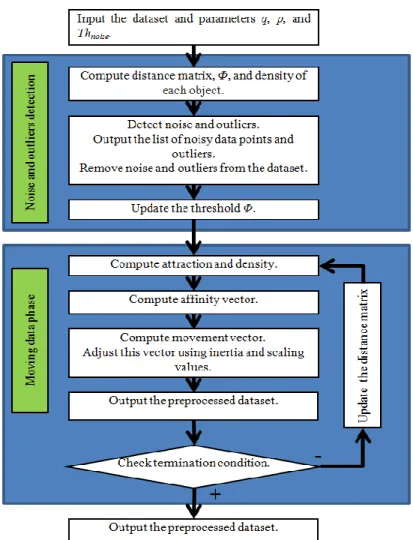
Figure 3.9 Outline of the D-IMPACT algorithm ... 23

Figure 3.10 An illustration of noisy points and outliers.. ... 24

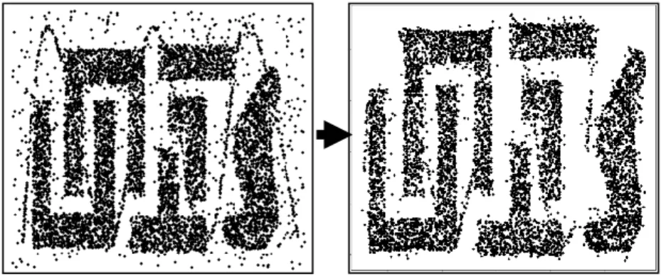
Figure 3.11 Illustration of the effect of noise removal in D-IMPACT.. ... 25

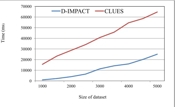
Figure 3.12 Processing times of D-IMPACT and CLUES on test datasets. ... 26

Figure 3.13 Visualizations of 2D datasets. ... 27

Figure 3.14 Visualization of the dataset DM130 preprocessed by D-IMPACT and CLUES ... ... 31

Figure 3.15 Visualization of the dataset MultiCL preprocessed by D-IMPACT and CLUES. ... ... 31

Figure 3.16 Visualization of two datasets t4.8k and t8.8k preprocessed by D-IMPACT ... 32

Figure 3.17 Visualizations of the dataset t4.8k preprocessed by CLUES using different values of k based on the size of the dataset.. ... 32

Figure 3.18 Visualization of the dataset Planet preprocessed by D-IMPACT and CLUES. ... 33 Figure 3.19 Visualization of the Iris dataset before and after preprocessing by D-IMPACT.

Visualization of the original dataset is shown in the bottom-left triangle.

v

Visualization of the dataset optimized by D-IMPACT is shown in the top-right

triangle. ... 35

Figure 3.20 Visualization of the first four features of the Wine dataset before and after preprocessing by D-IMPACT. Visualization of the original dataset is shown in the bottom-left triangle. Visualization of the dataset preprocessed by D-IMPACT is shown in the top-right triangle. ... 36

Figure 3.21 Visualization of the Iris and Wine datasets preprocessed by CLUES. ... 37

Figure 3.22 Dendrograms of the clustering results on the WTP dataset. ... 39

Figure 4.1 Clustering search results for the word “Kanazawa”.. ... 42

Figure 4.2 The rapid increasing of the number of dimensions and sparseness when the number of texts increases. ... 43

Figure 4.3 D-IMPACT algorithm degenerated the performance of clustering on text data.. 45

Figure 4.4 An illustration of WordNet’s structure. ... 47

Figure 4.5 Flowchart of SCF algorithm. ... 50

Figure 4.6 Algorithm for removing words which have extreme high document-frequency.. 52

Figure 4.7 Clustering algorithm for clustering words based on semantic similarity. ... 54

Figure 4.8 Algorithm for identifying keywords in each-document and selecting important representative words. ... 56

Figure 4.9 Histogram of semantic similarity between verb-verb using first k (k= 2 at the left, k = 3 at the right) concepts ... 59

Figure 4.10 Histogram of semantic similarity between noun-noun using first k (k= 2 at the left, k = 3 at the right) concepts. ... 59

Figure 4.11 Histogram of values of covariance matrix between important representative words in Enron dataset... 60

Figure 4.12 Comparison of clustering performances on UC Berkeley Enron and 20

newsgroups datasets.. ... 62

vi

List of tables

Table 3.1 Experiment datasets for IMPACT algorithm. ... 16

Table 3.2 Experiment datasets for D-IMPACT algorithm. ... 29

Table 3.3 Parameter sets of D-Impact for experiments.. ... 30

Table 3.4 The Index scores of clustering results using HAC on the original and preprocessed

datasets of IRIS and Wine. The best scores are in bold ... 37

Table 3.5 Index scores of clustering results using k-means on original and preprocessed

datasets of IRIS and Wine. The best scores are in bold.. ... 37

Table 3.6 Accuracy and precision values of noise and outlier detection on the Lung-cancer

dataset ... 40

Table 4.1 Characteristics of UC Berkeley Enron and 20 newsgroups datasets. ... 58

Table 4.2 Result of feature reduction by word clustering and SCF algorithm. ... 61

vii

Abbreviations

PCA = Principal Component Analysis

HAC = Hierarchical Agglomerative Clustering RI = Rand Index

aRI = adjusted Rand Index

LSI = Latent Semantic Indexing

WSD = Word Sense Disambiguation

viii

Acknowledgements

I want to express my gratitude to Prof. Kenji Satou for supervising this dissertation, and for numerous fruitful, serious, and enthusiastic discussions that initiated or improved many of the presented ideas and results. I am indebted to his guidance, patience, and mentorship.

I wish to thank Kanazawa University for providing me this scholarship. It created a change for me to explore and enjoy the life in Japan.

Finally I would like to thank all of my friends and my whole family, who supported me during

the time I get my PhD. in Kanazawa University.

ix

Abstract

Clustering is a process that divides data into groups (clusters) whose memberships are similar to each other than data objects belong to other groups This task is useful for manage, summarize, and understand the patterns underlying the data. Although it has a long history of development, there remain open problems, such as how to determine the number of clusters, the difficulty in identifying arbitrary shapes of clusters, and the curse of dimensionality. Preprocessing methods can help to solve those problems and hence improve the quality of clustering. In this study, we propose two data preprocessing algorithms called D-IMPACT and SCF algorithms. D-IMPACT algorithm has two phases. The first phase detects noisy and outlier data points based on the density, and then removes them. The second phase separates clusters by iteratively moving data points based on attraction and density. Our second work, the data preprocessing algorithm SCF, aims to reduce the number of dimensions without losing the semantic information stored in each feature for short text data. SCF algorithm has two phases: the first phase is doing pruning on to remove unnecessary words and replace semantically related words by a representative word. In the second phase, SCF algorithm transforms the data matrix into Semantic similarity Conceptual Feature (SCF) space, which presents the semantic similarity between keywords of each document and the concept underlying all the documents. Our experiment results show that D- IMPACT and SCF algorithms are able to improve the performance of the clustering algorithms performed on datasets preprocessed by them.

Keyword: data preprocessing, clustering, data point movement, feature reduction, semantic

similarity.

1

Dissertation introduction

1.1 Dissertation overview

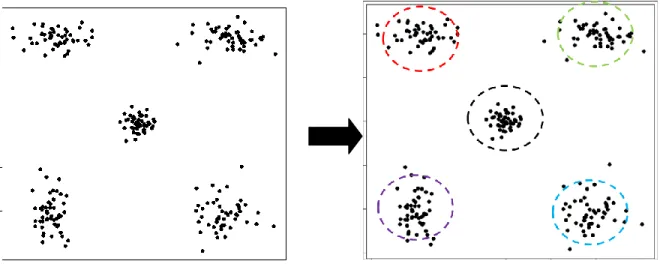
Clustering is a process that divides data into groups (clusters) whose memberships are similar to each other than data objects belong to other groups (Figure 1.1). Simply, clustering is the task that data objects are divided into groups whose memberships are similar to each other than data objects belong to other groups. Clustering is applied in many fields, such as: decision-making, machine-learning situations, document retrieval, image segmentation, bioinformatics, and finance. The discovered clusters can be used to explain the characteristics of underlying data, or server as the foundation for other data analysis techniques.

Figure 1.1 A simple example of clustering.

Although it has a long history of development, there remain open problems, such as how to

determine the number of clusters, the difficulty in identifying arbitrary shapes of clusters, and the

curse of dimensionality [1]. The majority of current algorithms perform well for only certain

types of data [2]. Therefore, it is not easy to specify the algorithm and input parameters required

to achieve the best result. In addition, it is difficult to evaluate the clustering performance, since

2

most of the clustering validation indexes are specified for certain clustering objectives [3].

Finding an appropriate algorithm and parameters is very difficult and requires a sufficient amount of experiment results. The datasets measured from real systems usually contain outliers and noise, and are, there-fore, often unreliable [4] [5]. Such datasets can impact the quality of cluster analysis. However, if the data have been preprocessed appropriately, for example, clusters are well-separated, dense and have no noise, the performance of the clustering algorithms may improve.

In this study, we propose two data preprocessing algorithms called D-IMPACT and SCF algorithm. D-IMPACT algorithm iteratively moves data points based on attraction and density to detect and remove noise and outliers, and separate clusters. SCF algorithm reduces the number of dimension and improves the quality of term frequency matrix based on semantic similarity and clustering. Our experiment results show that these methods are able to produce new datasets such that the performance of the clustering algorithm is improved.

1.2 Dissertation distribution

Chapter I is to present our research and contribution. Chapter II briefly presents the

background and challenges of clustering, then introduce the data preprocessing to overcome the

challenges in clustering. Chapter III introduces our first data preprocessing algorithm D-

IMPACT, which focuses on de-noising and separating clusters. Chapter IV presents SCF

algorithm, a semantic-based data preprocessing method, to reduce the number of feature and

improve the content presented in term frequency matrix. The dissertation is concluded in

Chapter V.

3

CHAPTER II

Clustering and data preprocessing for clustering

This chapter briefly presents the background of clustering and its challenges. We then introduce data preprocessing methods in order to deal with challenges in clustering.

2.1 Clustering

2.1.1 Background of clustering

As introduced above, clustering task organizes data objects into groups whose members are similar in some way. A cluster is therefore a collection of objects which are similar between them and are dissimilar to the objects belonging to other clusters. Clustering is applied in various fields, e.g., marketing (categorizes the customer), biology (classify the gene expression data), geography (identify the similar zones appropriate for exploitation) and so on.

Clustering has more than 50 years of development. Many clustering algorithms were proposed with different schemas and concepts [1]. The taxonomy of clustering techniques is not unique due to the different viewpoints of comparisons. Some algorithms are the combination of different techniques and concepts, therefore they can be classified to various classes. We only introduce common representative algorithms for each clustering technique’s class.

Partitioning clustering algorithm These clustering techniques attempt to break a dataset into k clusters by optimizing a given criterion. They usually repeat the iteration of finding the centroid of each cluster and assigning points to the centroids until the criterion is assumed maximized. k-means, k-medoids [1], and PAM [6] are simple examples of partitioning clustering algorithms.

Hierarchical clustering algorithm Hierarchical clustering algorithms start with each data

point belonging to one of the disjoint clusters, then merge the two most similar clusters, or

vice versa, start with the whole dataset then divide them to two most different cluster. Those

processes continue until stop conditions are satisfied. The clustering result is outputted as a

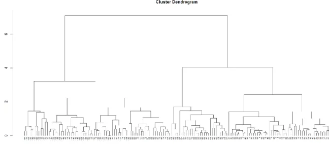
dendrogram (Figure 2.1). Some well-known algorithms for this class are Hierarchical

Clustering (HC) [1] and CURE [7].

4

Figure 2.1 An example of dendrogram.

Density based clustering algorithm Density-based clustering algorithms attempt to find dense regions separated from other regions that satisfy certain criteria related to density.

DBSCAN [8], the most popular Density based clustering algorithm, scans and finds all possible regions such that the size of the region is larger than minPts within the Esp radian.

The minPts and Esp parameter then become two specific characteristics for the algorithms belong to this class.

Grid based clustering algorithm Grid-based clustering algorithms limit the search space into segments (e.g., cubes, cells, and regions) according to attribute space. This type of clustering algorithm is proposed with the hope to get rid of the curse of dimensionality problem. CLIQUE [9], STING [10] are clustering algorithm feature this type of Grid-based clustering algorithms.

2.1.2 Challenges in clustering

Even though with a long history of research and development, there are still several challenges existed for clustering:

The number of clusters. Most of clustering algorithms require a priori specification number

of clusters. Others require a specific threshold or rely on a criterion to determine the number

of clusters.

5

High dimensionality. The different between objects belong to same clusters and ones belong to other clusters decease as the increasing of the number of dimensions. This problem makes similarity function loss its usefulness on discriminating data objects.

Clustering validation. Various criteria or indexes are employed to validate the clustering result. However, since there is no “best” criterion or index, the choice of volition function can highly affect the clustering result.

Noise and outlier. The datasets measured from real systems usually contain outliers and noise, and are, there-fore, often unreliable. Such datasets can impact the quality of cluster analysis.

Such problems can impact the quality of cluster analysis. However, if the data have been preprocessed appropriately, for example, clusters are well-separated, dense and have no noise, the performance of the clustering algorithms may improve. Data preprocessing is often used to perform such tasks.

2.2 Data preprocessing

Real world data usually contain noises and outliers, are high dimensional, hence, strongly impact the performance of clustering. To deal with such problems, data preprocessing methods are employed to improve quality of data and therefore, improve the performance of clustering.

The popular tasks of data preprocessing methods in clustering are:

Feature reduction. These methods represent the input space into a lower-space but still retain the variance of the data as possible. Principal Component Analysis (PCA) [11] is a well-known example for feature reduction methods. The concept of PCA is finding new principal components, which linear with variance of data, to reduce the number of dimension with minimal loss of information. Although PCA accounts for as much variance of the data as possible, clustering algorithms combined with PCA do not necessarily improve, and, in fact, often degrade, the cluster quality [12]. PCA essentially performs a linear transformation of the data based on the Euclidean distance between samples; thus, it cannot characterize an underlying nonlinear subspace.

Feature selection. Feature reduction methods represent the input space into a new space,

and hence, cause the loss of features in original space. In contrast to feature reduction,

feature selection methods try to select a subset of features in original space such that the

6

clustering performed on this space can be improved. Many feature selection methods for clustering are summarized in [13].

Noise and outlier removal. Noises and outliers greatly affect the performance of clustering.

Several clustering algorithms, i.e., single linkage hierarchal clustering, often miss-clusters outliers as clusters. Noises reduce the intercluster similarity, hence make clusters becomes not well-separated. A lot of methods were proposed in order to identify and remove noises and outliers to make the identification of clusters easier (Figure 2.2). A number of outlier removal methods are summarized in [14].

Figure 2.2 Illustration of the effect of noise removal

In this chapter, we introduce the background of clustering and data preprocessing for clustering. Several clustering and data preprocessing methods were introduced. In the next chapter, we will present our data preprocessing algorithm D-IMPACT in detailed.

7

CHAPTER III

Data preprocessing algorithm D-IMPACT

In this chapter, we describe the data preprocessing algorithm D-IMPACT based on concepts underlying the clustering algorithm IMPACT [15]. We aim to improve the accuracy and flexibility of the movement of data points in the IMPACT algorithm by applying the concept of density to various affinity functions. These improvements will be described in the subsequent subsections.

3.1 Gravity-based data preprocessing algorithm

Recent studies have focused on new categories of clustering algorithms which prioritize the application of data preprocessing. SHRINK, a data shrinking process, moves data points along the gradient of the density, generating condensed and widely separated clusters [16]. Following data shrinking, clusters are detected by finding the connected components of dense cells. The data shrinking and cluster detection steps are conducted on a sequence of grids with different cell sizes. The clusters detected at these cells are compared using a cluster-wise evaluation measurement, and the best clusters are then selected as the final result. In CLUES [17], each data point is transformed such that it moves a specific distance toward the center of a cluster. The direction and the associated size of each movement are determined by the median of the data point’s k nearest neighbors. This process is repeated until a pre-defined convergence criterion is satisfied. The optimal number of neighbors is determined through optimization of commonly used index functions to evaluate the clustering result generated by the algorithm. The number of clusters and the final partition are determined automatically without any input parameters, apart from the convergence stop criteria.

These two shrinking algorithms share the following limitations:

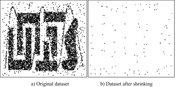
 The process of shifting toward the median of neighbors can easily fracture the cluster (Figure 3.1).

 The direction of the movement vector is not appropriate in specific cases. For example,

if the clusters are adjacent and differ highly in density, the median of the neighbors is

likely to be located on another cluster.

8

We introduce IMPACT, a clustering algorithm based on the simulation of gravity system:

moving data points under effect of attractive-force like values to form dense regions that can be easily identified as clusters. The data points movement in IMPACT algorithm can avoid the addressed problems. The next section will explain the algorithm in detailed.

Figure 3.1 Clusters are fractured after shrinking.

3.2 Clustering algorithm IMPACT 3.2.1 IMPACT algorithm

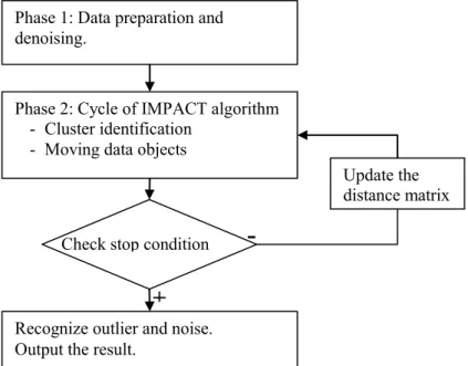
The IMPACT algorithm is based on the idea of gradually moving all objects closer to similar objects according to the attraction between them until the dataset becomes self- partitioned. The algorithm has two phases. The first phase is for normalizing and denoising the input dataset. In the second phase, IMPACT iteratively moves the data points and identifies clusters. The flowchart of IMPACT algorithm is described in Figure 3.2.

a) Original dataset b) Dataset after shrinking

9

Figure 3.2 Flowchart of the IMPACT algorithm A) Phase 1: Normalizing and denoising the input dataset.

The first step in this phase is to read the input data and normalize the numerical attribute values into the range [0,1]. The objective of this process is to avoid attributes with a wide

range of values dominating the clustering results. Each value in the dataset is modified as

x

x

x x x

..m rj rj r

..m r

..m rj ij r

ij

max ( ) min ( )

) ( min

1 1

1









 

.

The distance matrix is computed from this normalized dataset. The threshold Th is then computed from the maximum value of the distance matrix (i.e., longest distance).

The second step of this phase is denoising. Since we identify clusters only by grouping data objects according to the threshold Th, in noisy datasets, clusters linking at the border region can affect the recognition of clusters. However, if we simply move the data objects, noise might be reduced and the border regions become clearer, as the points move closer to their centroids and the gaps between clusters widen. The denoising step is controlled by a denoise-level parameter, which is the number of steps of moving data objects. The noisier a dataset is, the bigger this value should be. Figure 3.3 shows the effect of denoising.

Phase 1: Data preparation and denoising.

Phase 2: Cycle of IMPACT algorithm - Cluster identification

- Moving data objects

Check stop condition

Recognize outlier and noise.

Output the result.

-

+

Update the

distance matrix

10

a) Before denoising b) After denoising Figure 3.3 Effect of denoising

B) Phase 2: Repeating the cycle of identifying clusters and moving data objects until the stop condition is satisfied.

Moving data objects can improve the quality of identified clusters by increasing the similarities between similar data objects and the dissimilarities between clusters. Firstly, we describe how to compute the movement of a data object (movement vector).

Given a dataset

{

|

} with m data objects (vectors), our objective is to group m data objects into clusters without specifying their number. We assume that each data object is attracted by others via a natural force called attraction as in a physical system. There are three steps to compute the movement vector of a data object:

Computing the attraction and attractive vector between all data objects

As in physics, objects attract each other and move closer under the effect of an attractive force among them (attraction).

Attraction Attraction is a quantity that represents the attractive force between two data objects x

and x

:

p j i j

i

ij

x x x x

A distance ( , )

) 1 , (

attraction 



,

where p (p > 0) is a user specified parameter used to adjust the effect of attraction

between two data objects.

11

Attractive vector Attractive vector is an n-dimensional vector representing the attractive force between a data object and another data object caused by the attraction between them. Attractive vector av

= (av

, av

… av

) of x

for x

is computed as

) ..

1 (

|

|

1

n k A x x

x

av

x

r jr ir

ik jk

ijk

 



 



Computing the movement vector for each data object

The attractive forces shift objects, as represented by movement vector. The direction of the movement vector v

of x

is the summation of all attractive vectors of all other data objects to x

:





j ij

i

av

v

1

Computing the Inertia of each cluster and the Scale value for each movement vector.

The length of the movement vector should be calculated carefully. For the sake of higher clustering accuracy, the distance of movement (magnitude of the movement vector) should not be too long. However, if the distance of the movement is too short, the clustering process will be slow. In addition, after data objects form a cluster, they do not need to move so much. Based on these considerations, the movement is adjusted by two values:

Inertia If x

belongs to a cluster C

, its movement vector v

is adjusted as )

1

(

i

i

v I

v    ,

where I

is the Inertia of cluster C

. The Inertia avoids clusters from moving too quickly and incorrectly merging.

Scale Because the threshold value Th is used during the clustering step, the appropriate magnitude of each movement vector should be no greater than Th.

Scale, a value used to adjust the length of movement vector, is computed as

|) (|

max

v

Scale Th





.

12

After adjustment, all movement vectors are guaranteed not to cross the scanning field of the nearest objects. It is therefore clear that the movement of data objects retains the global and local structure of the cluster: the Inertia ensures clusters do not merge easily, while computation of all the attractions affecting one data object retains the global balance.

Finally, data objects are moved as

i i

i

x Scale v

x    .

The movement increases the similarity between close objects and the dissimilarity between groups by increasing the distance of their borders. Figure 3.4 summarizes the steps to move data objects.

Next, clusters are identified. Cluster identification is the process by which indistinguishable data objects are grouped together. The pseudo code in Figure 3.5 presents the steps in this process. If the distance between two objects is less than Th, they are linked and form a group. The threshold Th used in the grouping step is computed as

e maxDistanc q

Th   _,

j i j

i

,x x ,x

x e

maxDistanc  max(distan ce ( ))  ,

where q is a parameter specified by the user to compute Th, the threshold value to determine whether two data objects are indistinguishable. For example, if q = 0.05, we can say that two data objects are indistinguishable if their difference is 5% less than the distance between the most different pair. Although all data objects are assigned to groups, not all groups can be considered as clusters. A group G is a cluster if it satisfies the condition

rSize min_Cluste

G 

,

where min_ClusterSize is a threshold used to eliminate small groups.

The iterative process stops when it meets the stop condition. The stop condition of the IMPACT algorithm can be satisfied in many ways, and not just when all data objects are clustered. Below are common stop conditions that are used for different objectives.

A given percentage of data objects have been clustered When all or most data objects

are clustered, we can stop the cycle and deal with unclustered objects later.

13

The magnitude of the longest movement vector is sufficiently small (e.g., less than Th or a user specified parameter) Data objects in dense regions are usually clustered quickly, while noisy objects and outliers are not attracted greatly by clusters.

This concept is employed by IMPACT to detect outliers and noise effectively. After detecting all clusters, outliers, and noise, the final clustering result is output.

Hence, we can see that the IMPACT algorithm works by iterating the grouping and moving

of data objects until the dataset is self-partitioned. To evaluate the performance of IMPACT

algorithm, we tested it on datasets with different characteristics. The results will be presented in

the next section.

14

Figure 3.4 Pseudo code of moving data points Input

x: data points p: input parameter Output:

x: data points after moving Algorithm:

compute attraction matrix:

p j i j

i

ij

x x x x

A distance ( , )

) 1 , (

attraction 



compute attractive vectors:

) ..

1 (

|

|

1

n k A x x

x

av

x

r jr ir

ik jk

ijk

 



 



av

= (av

, av

… av

) compute movement vector:





j ij

i

av

v

1

compute Inertia for each cluster:

sterSize largestClu I

| C

|



for each movement vector x

if x

C

then

adjust x

’s movement vector as:

) 1

(

i i j

i

C v v I

x     

compute the Scale value:

|) (|

max

v

Scale Th





end if end for

move all data points:

i i

i

x Scale v

x   

end;



15

Figure 3.5 Pseudo code of cluster identification

3.2.2 Experiment result

In this section, we evaluate the performance of IMPACT and demonstrate its effectiveness for different types of data distributions. We use six synthetic datasets, two datasets used in the paper presenting the Chameleon algorithm, two datasets from the UCI Machine Learning Repository, and one text dataset. We firstly introduce these eleven datasets used in this experiment.

The six synthetic datasets are denoted DS1 to DS5, and DS8. DS1 and DS2 are hierarchical datasets. DS3 and DS4 contain clusters with different densities and sizes. DS5 includes many disjointed clusters (142 clusters) to demonstrate that IMPACT works well with a large number of clusters. DS6 and DS7 [18] are extremely difficult to cluster: they contain clusters with different shapes, noise and outliers. DS6 has a chain connecting all clusters (i.e., the single-link effect), while DS7 contains clusters with different arbitrary shapes. The gaps between clusters are small and filled with noise. DS8 is a simple hard clustering dataset that includes 100 points generated

Input

x: data points

Th, min_ClusterSize: input parameter Output:

C: set of clusters Algorithm:

l = 0; V = ∅ ; for each x

∉ V then

S = x

; G = ∅ ;

while S ≠ ∅ do

Randomly take x

out of S;

G = G {x

} V = V {x

}

for each x

∉ V do

if distance(x

,x

)<Th S = S {x

} end if

end for end while

if |G| ≥ min_ClusterSize then l++;

C

= G

end if

end for

16

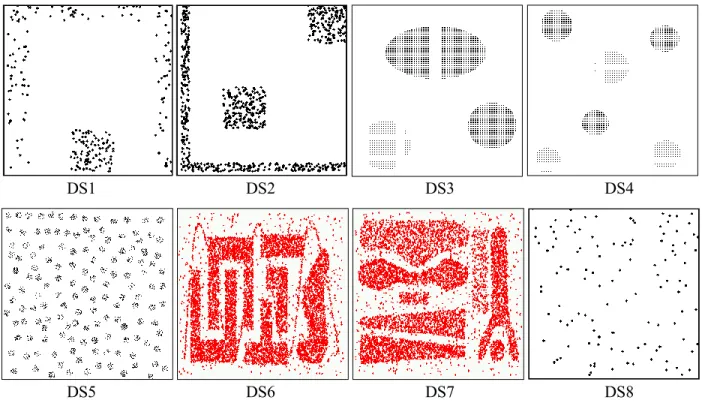
randomly, and three 10 point clusters placed in three corners of the dataset. DS8 does not have any “natural” clusters, so the clustering results could differ depending on the cluster validity.

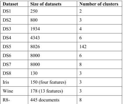
DS8 is suitable for testing the validity of the clustering algorithm. Figure 3.6 presents all datasets from DS1 to DS8 in two-dimensional plots. Wine and Iris are commonly used datasets taken from the UCI Machine Learning Repository [19]. R8- [20] is a sub collection of the Reuters-21578 dataset. These datasets characterize different problems in clustering. Table 3.1 gives the sizes of all datasets and the numbers of desired clusters (the correct clustering results) for them.

Table 3.1 Experiment datasets for IMPACT algorithm Dataset Size of datasets Number of clusters

DS1 250 2

DS2 800 3

DS3 1934 4

DS4 4343 6

DS5 8026 142

DS6 8000 6

DS7 8000 8

DS8 130 3

Iris 150 (four features) 3 Wine 178 (13 features) 3

R8- 445 documents 8

17

DS1 DS2 DS3 DS4

DS5 DS6 DS7 DS8

Figure 3.6 Illustrations of datasets from DS1 to DS8

The results of IMPACT are presented and analysed in below. More detailed results and comparisons with other algorithms can be found on the literature of IMPACT algorithm.

Cluster identifying ability To demonstrate the ability of the IMPACT algorithm to identify

clusters, we performed clustering on DS1, DS2, DS3, DS4, DS5, DS6, and DS7, which are

datasets with different cluster types. The results are shown in Figure 3.7. Clustering results

obtained from DS1 and DS2 datasets with IMPACT demonstrate that IMPACT can cluster

hierarchical datasets effectively. Figure 17 shows results obtained from DS3 and DS4 using

IMPACT with default parameters. The clustering results show that IMPACT is not affected

by the size and density of clusters. In case of DS 5, IMPACT identified correctly all 142

clusters of DS5. The clustering results of the last two datasets DS6 and DS7, shown in

Figure 19, are similar to the results reported in the literature [21]: most clusters are the same

but in the case of DS7, IMPACT breaks the marked cluster into two smaller clusters owing

to the presence of some low-density regions within. The results demonstrate that IMPACT is

quite effective in finding clusters of arbitrary shape, density, and orientation.

18

DS1 DS2 DS3 DS4

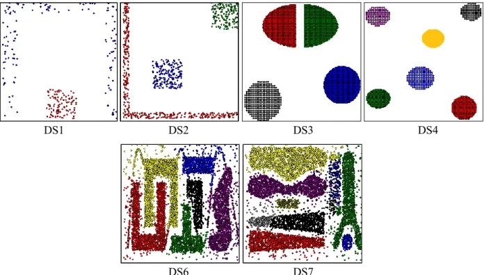
DS6 DS7

Figure 3.7 Clustering results for DS1, DS2, DS3, DS4, DS6, and DS7 using IMPACT algorithm Parameter sensitivity of the IMPACT algorithm One of the most critical clustering problems is sensitivity to input parameters. To obtain accurate clustering results, we usually need to estimate the best value of the parameters for the given dataset. The IMPACT algorithm is designed to overcome this problem. We ran IMPACT with default parameters (p

= 2, q = 0.05, min_ClusterSize = 20%) on DS8. Clustering results obtained by running IMPACT with different parameter values of p and q are shown in Figure 3.8. It is seen how with different values of p and q, IMPACT produces the same results with a dataset with not well-separated clusters. This result suggests that the IMPACT algorithm is not parameter sensitive.

Figure 3.8 Clustering results for DS8 using IMPACT

19

Practical datasets The IMPACT algorithm not only works effectively with two-dimensional datasets but also produces accurate results when dealing with practical datasets. We used two common datasets from the UCI Machine Learning Repository (Wine and Iris) and one text dataset (R8-) for validation. In the case of the Wine and Iris datasets, the IMPACT algorithm found the correct number of clusters in most tests and archive highest Rand index scores [22]

in most of cases. The text dataset R8- needs to be preprocessed before clustering. We used a Perl program to stem nouns and verbs to generate the dictionary and feature vector from R8-.

However, because of the high dimension of feature vectors, IMPACT failed to identify the clusters in the dataset. To avoid this problem, we applied PCA to reduce the number of features, and then employed IMPACT for clustering. Even IMPACT could detect seven clusters only, but its result is remarkable because (1) IMPACT did not require the correct number of clusters and (2) the F

score [22] for IMPACT (0.87) is higher than other results in the literature [23] and [24].

In all the experiments described above, our algorithm was able to identify clusters accurately for most of the datasets and was insensitive to the choice of parameters. However, there are several limitations existed for IMPACT algorithm:

 The datasets are not completely denoised.

 In several cases, small parts of clusters are merged.

 IMPACT takes long processing time to cluster the data.

In this study, we propose a data preprocessing algorithm named D-IMPACT (Density- IMPACT) [25] to overcome the limitation of gravity-based preprocessing algorithms by utilizing the idea of IMPACT algorithm and the concept of density [8]. An advantage of our algorithm is its flexibility in relation to various types of data; it is possible to select an affinity function suitable for the characteristic of the dataset. This flexibility improves the quality of cluster analysis even if the dataset is high-dimensional and non-linearly distributed, or includes noisy samples.

3.3 Data preprocessing algorithm D-IMPACT

In this section, we describe the data preprocessing algorithm D-IMPACT based on concepts

underlying the IMPACT algorithm. We aim to improve the accuracy and flexibility of the

20

movement of data points in the IMPACT algorithm by applying the concept of density to various affinity functions. These improvements will be described in the subsequent subsections.

3.3.1 Movement of data points

The main difference between the data movement in D-IMPACT and IMPACT algorithms is that the movement of data points can be varied by the density functions, the attraction functions, and an inertia value. This helps D-IMPACT detect different types of clusters and avoid many common clustering problems. In this subsection, we describe the scheme to move data points in D-IMPACT. We assume that the dataset has m samples and each sample is characterized by n features. We also denote the feature vector of the i

sample by x

.

3.3.1.1 Density

We use two formulae to compute the density of a data point based on its neighbors, which are defined as data points located within a radius Φ. This density is calculated with and without considering the distance from the data point to its neighbors. We define the density δ

for the data point x

as

, ) ( den

i

x

δ 

where den(xi) is one of following density functions:

|, ) (

| ) (

den

x

 NN x

) , , distance(

| ) ( ) |

( den

) (

2

  





 







 

 _i

j NNx

x i j

i

i

x x

x x NN

where NN(x

) is the set of neighbors of x

and |NN(x

)| is the number of neighbors. Unlike the density function den

, the density function den

considers not only the number of neighbors, but also the distance between them to avoid issues relating to the choice of threshold value, Φ. In a practical application, we scale the density to avoid scale differences arising from the use of specific datasets as follows:

) . ( max

δ δ δ

..m j j

i i





21

3.3.1.2 Attraction

In our D-IMPACT algorithm, the data points attract each other and one other closer. We define the attraction of data point x

caused by x

as

distance( , )

aff(

) distance(

) 0 ( attraction

 





 

 x ,x if x ,x ) Φ

Φ ,x x ,x if

x A

j i j

i

j i j

i ij

where aff(x

,x

) is a function used to compute the affinity between two data points x

and x

. This quantity ignores the affinity between neighbors. The affinity can be computed using the

following formulae:

) , , ( distance ) 1

, (

aff

j i j

i

x x x

x 

) , , ( distance ) 1

, (

aff

j i j

j

i

x δ x x

x  

) , , ( distance

1 )

, max(

) , ) min(

, (

aff

j j i

i j i j

i

δ δ x x

δ x δ

x  

) . , ( distance

1 )

, max(

) , ) min(

, (

aff

j i j

i j i j

j

i

δ δ x x

δ δ δ

x

x   

These four formulae have been adopted to improve the quality of the movement process in specific cases. The function aff

, used in IMPACT, considers the distance between two data points only. The function aff

considers the effect of density on the attraction; highly-aggregated data points cause stronger attraction between one another than sparsely-scattered data points.

This technique can improve the accuracy of the movement process. The function aff

considers

the difference between the densities of two data points; two data points attract each other more

strongly if their densities are similar. This can be used in the case where clusters are adjacent but

have differing densities. The function aff

is a combination of aff

and aff

. The parameter p is

used to adjust the effect of the distance to the affinity. Attraction is the key value affecting the

computation of the movement vectors. For each specific problem in clustering, an appropriate

attraction computation can help D-IMPACT to correctly separate clusters.

22

Under the effect of attraction, two data points will move toward each other. This movement is represented by an n-dimensional vector called the affinity vector. We denote a

as the affinity vector of data point x

caused by data point x

. The k

element of a

is defined as

).

..

1 (

|

|

1

n k A x x

x

a

x

r jr ir

ik jk

ijk

 



 



The affinity vector is a component used to calculate the movement vector.

3.3.1.3 Inertia value

To shrink clusters, D-IMPACT moves the data points at the border region of original clusters to the centroid of the cluster. Highly aggregated data points, usually located around the centroid of the cluster, should not move too far. In contrast, sparsely-scattered data points at the border region should move to the centroid quickly. Hence, we introduce an inertia value to adjust the magnitude of each movement vector. We define the inertia value I

of data point x

based on its density

by

. 1 δ

I

 

3.3.1.4 Data point movement

D-IMPACT moves a data point based on its corresponding movement vector. The movement vector v

of data point x

is the summation of all affinity vectors that affect the data point x

,







j ij

i

a

v

where a

is the affinity vector. The movement vectors are then adjusted by the inertia value and scaled by s, which is a scaling value used to ensure the magnitude does not exceed a value Φ, as in the IMPACT algorithm. This scaling value is given by

||) . (||

max

v

s Φ





1

In the case of sparse datasets, neighbor detection based on a scanning radius usually fails.

Therefore, most of data points will have a density equal to 1. Hence, we replace the formula

used to compute the inertia value with

23

Finally, each data point is moved using

)

,

1 ( )

(k i k i i

i

x s I v

x 

  

where x

is the coordinate of data point x

in the previous iteration, and x

is the coordinate of data point x

in this iteration. We propose the algorithm D-IMPACT based on this scheme of moving data points.

3.3.2 D-IMPACT algorithm

D-IMPACT has two phases. The first phase detects noisy and outlier data points, and then removes them. The second separates clusters by iteratively moving data points based on attraction and density functions. Figure 3.9 shows the flow chart of the D-IMPACT algorithm.

The algorithm will be explained in detailed in next sections.

Figure 3.9 Outline of the D-IMPACT algorithm

24

3.3.2.1 Noisy points and outlier detection

First, the distance matrix is calculated. The density of each data point is then calculated by one of the formulae defined in the previous subsection. The threshold used to identify neighbors is computed based on the maximum distance and the input parameter q, and is given by

, e maxDistanc q

Φ  

where maxDistance is the largest distance between two data points in the dataset.

The next step is noise and outlier detection. An outlier is a data point significantly distant from the clusters. We refer to data points which are close to clusters but do not belong to them to as noisy points, or noise, in this manuscript. Both of these data point types are usually located in sparsely-scattered areas, that is, low-density regions. Hence, we can detect them based on density and the distance to clusters. We consider a data point as noisy if its density is less than a threshold Th

, and it has at least one neighbor which is noisy or a cluster-point (with the latter defined as a data point whose density is larger than Th

). An outlier is a point with a density less than Th

that has no neighbor which is noisy or a cluster-point. Figure 3.10 gives an example of noise and outlier detection.

Figure 3.10 An illustration of noisy points and outliers.

Both outliers and noisy points are output and then removed from the dataset. The

effectiveness of this removal is shown in Figure 3.11. The value Φ is then recalculated as the

dataset has been changed by the removal of noise and outliers. When this phase is complete, the

movement phase commences.

25

Figure 3.11 Illustration of the effect of noise removal in D-IMPACT.

3.3.2.2 Moving data points

In this phase, the data points are iteratively moved until the stop criterion is met. The distances and the densities are calculated first, after which, we compute the components used to determine the movement vectors: attraction, affinity vector, and the inertia value. We then employ the movement method described in the previous section to move the data points. The movement shrinks the clusters to increase their separation from one another. This process is repeated until the stop condition is satisfied. In D-IMPACT, we adopt various stop criteria as follows:

 Stop after a fixed number of iterations controlled by the parameter n

.

 Stop based on the average of the densities of all data points.

 Stop when the magnitudes of movement vectors have decreased significantly compared to the previous iteration.

When this phase is complete, the preprocessed dataset is output. The new dataset contains separated and shrunk clusters, with noise and outliers removed.

3.3.2.3 Complexity

D-IMPACT is a computationally-efficient algorithm. The cost of computing m

affinity vectors is O(m

n). The complexity of the computation of movement vectors is O(mn). Therefore, the overall cost of an iteration is O(m

n). We see, based on our experiments, that the number of iterations is usually small and does not have significant impact on the overall complexity.

Therefore, the overall complexity of D-IMPACT is O(m

n).

We measured the real processing time of D-IMPACT on 10 synthetic datasets. For each dataset, the data points were randomly located (uniformly distributed). The sizes of the datasets varied

26

from 1000 to 5000 samples. These datasets are included in the supplement. We compared D- IMPACT with CLUES using these datasets. D-IMPACT was employed with the parameter n

set to 5. For CLUES, the number of neighbors was set to 5% of the number of samples and the parameter itmax was set to 5. The experiments were executed using a workstation with a T6400 Core 2 Duo central processing unit running at 2.00 GHz with 4 GB of random access memory.

Figure 3.12 shows the advantage in speed of D-IMPACT in relation to CLUES.

Figure 3.12 Processing times of D-IMPACT and CLUES on test datasets.

0 10000 20000 30000 40000 50000 60000 70000

1000 2000 3000 4000 5000

T im e (m s

Size of dataset

D-IMPACT CLUES

27

3.4 Experiment result

In this section, we compare the effectiveness of D-IMPACT and the shrinking function of CLUES (in short, CLUES) on different types of datasets.

3.4.1 Datasets and method

3.4.1.1 Two-dimensional datasets

To validate the effectiveness of D-IMPACT, we used different types of datasets: two dimensional (2D) datasets taken from the Machine Learning Repository (UCI), and a microarray dataset. Figure 3.13 shows the 2D datasets used.

Figure 3.13 Visualizations of 2D datasets.

The 2D datasets are DM130, t4.4k, t8.8k, multiCL, and Planet. They contain clusters with different shapes, densities and distributions, as well as noisy samples. The DM130 dataset has 130 data points: 100 points are generated randomly (uniformly distributed), and then three clusters, where each cluster comprises ten data points, are added to the top-left, top-right and

a) DM130 b) MultiCL

c) t4.8k d) t8.8k e) Planet

28

bottom-middle area of the dataset (marked by red rectangles in Figure 3.13a). The MultiCL dataset has a large number of clusters (143 clusters) scattered equally. Two datasets, t4.8k and t8.8k [18], used in the analysis of the clustering algorithm Chameleon [21], are well-known datasets for clustering. Both contain clusters of various shapes and are covered by noisy samples.

Clusters are chained by the single-link effect in the t4.8k dataset. The clusters of the Planet dataset are adjacent, but differ in density. These datasets encompass common problems in clustering.

3.4.1.2 Practical datasets

The practical datasets are more complex than the 2D datasets, i.e., the high dimensionality can greatly impact the usefulness of the distance function. We used the Wine, Iris, Water-treatment plant (WTP), and Lung-cancer (LC) datasets from UCI, as well as the dataset GSE9712 from the Gene Expression Omnibus [26] to test D-IMPACT and CLUES on high-dimensional datasets.

The datasets are summarized in Table 3.2. The Iris dataset contains three classes (Iris Setosa, Iris

Versicolour, Iris Virginica), each with 50 samples. One class is linearly separable from the other

two; the latter are not linearly separable from each other. The Wine dataset (178 samples, 13

attributes), which are the results of chemical analysis of wines grown in the same region in Italy,

but derived from three different cultivars, include three overlapping clusters. The WTP dataset

(527 samples, 38 attributes) includes the record of the daily measures from sensors in an urban

waste water treatment plant. It is an imbalanced dataset - several clusters have only 1-4 members,

corresponding to the days that have abnormal situations. The lung-cancer (LC) dataset (32

samples, 56 attributes) describes 3 types of pathological lung cancers. Since the Wine, WTP, and

LC datasets have attributes within different ranges, we perform scaling to avoid the domination

of wide-range attributes. The last dataset we use is a gene expression dataset, GSE9712, which

contains expression values of 22283 genes from 12 radio-resistant and radio-sensitive tumors.

29

Table 3.2 Experiment datasets for D-IMPACT algorithm.

Dataset Size of datasets

Number of

features Number of clusters

DM130 130 2 3

MultiCL 8026 2 143

t4.8k 8000 2 8

t8.8k 8000 2 8

Planet 719 2 2

Iris 150 4 3

Wine 178 13 3

WTP 527 38 13

LC 32 56 3

GSE9712 12 22283 4

3.4.1.3 Validating methods

For a fair comparison, we employed CLUES implemented in R [27] and varied the number of

neighbors k (from 5% to 20% of the number of samples) for different datasets. For D-IMPACT,

we used the default parameter set (q = 0.01, p = 2, aff

, den

Th

= 0, n

= 2) with some

modifications. The complete parameter set is described in Table 3.3. We compared the

differences between the preprocessed datasets and the original datasets using 2D plots. However,

it is difficult to visualize the high-dimensional datasets using only 2D plots. For this reason, we

compared the two algorithms by using a plot showing several combinations of features. Further,

to evaluate the quality of the preprocessing, we compared the clustering results for the datasets

preprocessed by D-IMPACT and CLUES. We used two evaluation measures, the Rand Index

and adjusted Rand Index (aRI) [22]. Hierarchical agglomerative clustering (HAC) was used as

the clustering method [1]. We used the Wine, Iris, and GSE9712 datasets to validate the

clustering results, and the WTP and LC datasets to validate the ability of D-IMPACT to separate

outliers from clusters.