Inflationary models in supergravity with inflaton in a vector multiplet, and spontaneous breaking of supersymmetry and R-symmetry after inflation

multiplet, and spontaneous breaking of supersymmetry and R-symmetry after inflation

Yermek Aldabergenov

Department of Physics

Graduate School of Science and Engineering Tokyo Metropolitan University

Thesis submitted in partial fulfillment for the degree of Doctor of Philosophy in Physics

2018

Abstract 6

Introduction 7

1 The Standard Model 9

1.1 Quantum field theory overview . . . . 9

1.1.1 Scalar field . . . . 9

1.1.2 Dirac spinor . . . . 12

1.1.3 Abelian gauge field . . . . 13

1.1.4 Non-abelian gauge field . . . . 14

1.1.5 Interactions and perturbation theory . . . . 16

1.1.6 Renormalization . . . . 22

1.2 Standard Model particles . . . . 24

1.3 Spontaneous electroweak symmetry breaking . . . . 27

1.4 Problems of the Standard Model . . . . 30

2 Supersymmetry and MSSM 31 2.1 Rigid (global) supersymmetry . . . . 31

2.1.1 Wess-Zumino model . . . . 32

2.1.2 Superspace and Superfields . . . . 34

2.1.3 Supersymmetric abelian gauge theory . . . . 37

2.1.4 Supersymmetric non-abelian gauge theory . . . . 38

2.2 Supergravity . . . . 38

2.2.1 Superfields in curved superspace . . . . 39

2.2.2 Chiral theory . . . . 41

2.2.3 Gauge theory . . . . 43

2.3 Minimal Supersymmetric Standard Model . . . . 44

2.3.1 ”Soft” SUSY breaking terms . . . . 46

2.3.2 Spontaneous electroweak symmetry breaking in MSSM . . . . 46

2.3.3 Higgs mixing . . . . 47

2.3.4 Sparticle mixing . . . . 48

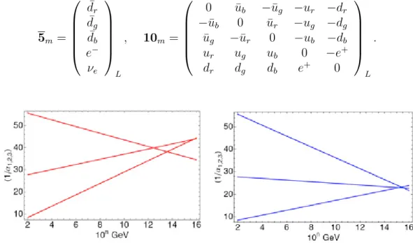
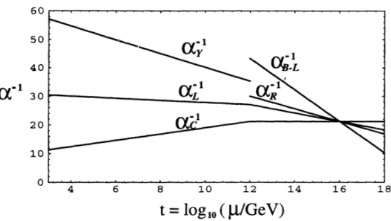
3 Grand Unified Theories 50 3.1 SU (5) unification . . . . 50

3.2 Flipped SU (5) . . . . 51

3.3 SO(10) models . . . . 52

3.4 E 6 models . . . . 53

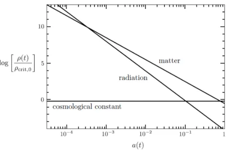
4 Standard Cosmology 55 4.1 FLRW universe . . . . 55

4.1.1 Composition of the Universe . . . . 56

4.1.2 Thermal history . . . . 57

4.1.3 Cosmological redshift . . . . 59

4.1.4 Horizons . . . . 59

4.2 Problems of Standard Cosmology . . . . 60

5 Inflationary Cosmology 61 5.1 Chaotic inflation . . . . 62

5.1.1 Slow-roll conditions . . . . 62

5.1.2 m ² φ ² -inflation . . . . 63

5.1.3 Starobinsky inflation . . . . 64

5.2 Graceful exit and reheating . . . . 65

5.2.1 Parametric resonance . . . . 66

5.3 Inflation and cosmic perturbations . . . . 67

5.3.1 Classification of perturbations . . . . 67

5.3.2 Scalar perturbations . . . . 68

5.3.3 Tensor perturbations . . . . 69

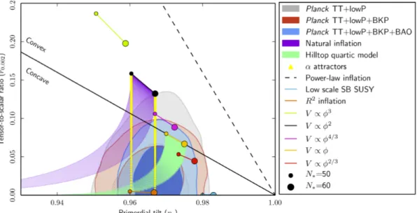
5.4 Observational constraints on inflationary models . . . . 69

6 Inflation in supergravity 71 6.1 Difficulties of embedding inflation into supergravity . . . . 71

6.2 F-term inflationary models . . . . 72

6.2.1 m ² φ ² -inflation . . . . 72

6.2.2 Hybrid inflation . . . . 73

6.3 D-term inflationary models . . . . 74

6.3.1 Quartic potential . . . . 74

6.3.2 D-term inflation with a massive vector multiplet . . . . 75

7 Inflation with inflaton in a vector multiplet and SUSY breaking 77 7.1 Non-minimal coupling of vector and chiral multiplets . . . . 77

7.2 Vacuum solution . . . . 80

7.3 Stability of the vacuum . . . . 82

7.4 Adding a cosmological constant . . . . 82

7.5 Massless vector multiplet and Higgs mechanism . . . . 83

7.6 Polonyi-Starobinsky model . . . . 86

7.7 Improved PS model with FI term . . . . 87

Conclusion 89

Acknowledgements 90

Bibliography 91

We consider inflationary model building in the framework of N = 1 supergravity, where the in- flaton scalar field belongs to a massive vector multiplet, and supersymmetry (and R-symmetry) is spontaneously broken after inflation. We show that it is possible to obtain a Minkowski and de Sitter vacua that are stable. We also reformulate our models as the U (1) gauge theories coupled to a Higgs chiral superfield, which in the minimal case corresponds to the standard U(1) Higgs setup. Finally, we focus on a specific representative of our class of models (called Polonyi-Starobinsky supergravity), that leads to the Starobinsky inflationary potential. We discover that the simplest known way to obtain the Starobinsky potential leads to instability, and find a way to remove it by adding a Fayet-Iliopoulos term. This leads to a modification of the previously found Polonyi vacuum.

Throughout the thesis, various connections of the conducted research to the Standard Model

(SM) of elementary particles, supersymmetry (SUSY) and supergravity, the Minimal Super-

symmetric Standard Model (MSSM), the supersymmetric Grand Unified Theories (GUT), the

Standard Cosmology (SC), cosmological inflation and superstrings are also discussed.

The inflationary paradigm solves initial-condition problems of the pre-inflationary cosmology (like e.g. the flatness problem, the horizon problem, the monopole problem) and remarkably agrees with CMB observations (COBE, WMAP, PLANCK). On the other hand, supergravity (or SUGRA for short), as well as its flat-space-time limit – rigid supersymmetry (SUSY), is a well-motivated framework for building UV-extensions of the Standard Model. Moreover, it is a necessary step if one considers unification of the Standard Model and General Relativity in the only known consistent framework of quantum gravity - superstring theories. Supersymmetry, if exists, cannot be exact, it must be spontaneously broken at some high-enough scale in order to generate large masses of superpartners of the Standard Model particles, as we do not see them at presently available energies. One can build a theory with various numbers (N) of supersymmetries, that would result in several distinct superpartners of the same particle. For instance, in 4 space-time dimensions, maximum number of supersymmetries for a gauge theory (where particle spin is no higher than 1) is N = 4, while for supergravity (where maximal spin is 2), N = 8. However, N > 1 supersymmetric theories are non-chiral, and for that reason they cannot be used as immediate extensions of the Standard Model, which is a chiral theory.

One of the most promising candidates for beyond-the-Standard-Model theory is the Minimal Supersymmetric Standard Model, which implements N = 1 supersymmetry. This motivates us to consider inflationary model building in the framework of N = 1 supergravity. However, realising inflationary potentials in supergravity was met with difficulties. One of them, called the η-problem, is related to the dangerous exponential factor in the F-term potential, which leads to the large effective mass of the would-be inflaton, and ruins the slow-roll regime required for successful inflation. Another problem arises if we assume that inflation was caused by a chiral superfield. Since the lowest component of a chiral superfield is a complex scalar, it provides two real degrees of freedom, one of which should be stabilised while the other drives the inflation. These problems can be avoided in various ways, one of which is to identify the inflaton with the real scalar component of a massive vector multiplet. Thus, there is no need for stabilisation, and since the inflationary potential comes from the D-term, this resolves the η-problem.

In generic inflationary models, although supersymmetry is spontaneously broken during infla- tion (since either D- or F-term potentials must have non-vanishing effective values), in the end of the inflation it is restored, and thus must be broken again by some mechanism.

In Chapter 1 we briefly review the main features of the Standard Model of particle physics.

In Chapter 2 we first introduce N = 1 supersymmetry, both global and local, then we show

how to apply global supersymmetry to the Standard Model. The resulting model is a very good candidate for beyond-the-Standard-Model theory, called the Minimal Supersymmetric Standard Model (MSSM). One of its features is the exact unification of its extrapolated coupling constants, which gives rise to the idea of Grand Unified Theories (GUT). We will discuss several candidate GUT models in Chapter 3.

The second half of the dissertation, devoted to cosmology, starts with the review of the Standard Cosmological Model (Chapter 4). In the end of Chapter 4 we review the problems of the pre-inflationary cosmology, and give motivation to introduce the idea of inflation. Chapter 5 is devoted to inflationary cosmology, where we review the simplest models, discuss particle production after inflation, and show the observational constraints on inflationary models. In Chapter 6 we consider embedding inflationary models in supergravity (local supersymmetry) by giving simple examples. Finally, in Chapter 7 we focus on the main goal of this dissertation, which is to (minimally) connect inflation, supergravity, and supersymmetry breaking after inflation, in a particular class of models. This is followed by conclusions where we summarise the main achievements of the research.

This research was conducted in collaboration with Associate Professor Sergei V. Ketov. The

main results were published in [1, 2].

The Standard Model

This chapter summarises basic information about Quantum Field Theory (QFT) and the Stan- dard Model (SM) of elementary particles along the lines of textbooks [3, 4, 5, 6].

1.1 Quantum field theory overview

In classical field theory the basic objects are fields: functions defined over some region of space.

Classical fields can be used to describe phenomena in classical physics, such as gravity or electromagnetism. However, to describe physics on subatomic scales, the need for the new class of theoretical framework arises, which is called quantum physics. We are particularly interested in its prominent representative called quantum field theory (QFT).

In QFT instead of classical fields one works with quantum fields, which are operator-valued functions. Quantum fields, in turn, act on a Fock space of all possible states, which is defined as a direct sum of 1, 2, ..., n-particle Hilbert spaces

H = H ₀ ⊕ H ₁ ⊕ H ₂ ⊕ ... ⊕ H _n . (1.1)

A quantum field can be obtained by the quantization procedure of a classical field, depending on the type of that field.

1.1.1 Scalar field

Let us start with the simple example of a real massive scalar field. Quantization of such a field corresponds to promoting a classical scalar field φ(x) described by the Lagrangian

L = − 1

2 ∂ _µ φ(x)∂ ^µ φ(x) − 1

2 m ² φ ² (x) , (1.2)

and obeying Klein-Gordon equation,

( − m ² )φ(x) = 0 , (1.3)

to an operator, which can be decomposed as ¹ φ(x) =

Z d ³ p

2E _p (2π) ³ a _p e ^ipx + a ^† _p e ^−ipx

, (1.4)

where px ≡ p µ x ^µ , E p = p

p ² + m ² is the energy, and a p and a ^† _p are annihilation and creation operators, respectively, which create or annihilate spin-0 excitations (particles) with momentum p of the corresponding field at point x in spacetime. They satisfy commutation relations

[a p , a q ] = [a ^† _p , a ^† _q ] = 0 , (1.5) [a _p , a ^† _q ] = 2E _p (2π) ³ δ ³ (p − q) , (1.6) which come from equal-time canonical commutation relations for φ(x) and its conjugate mo- mentum π(x) ≡ φ(x): ˙

[φ(t, x), φ(t, y)] = [π(t, x), π(t, y)] = 0 , (1.7) [φ(t, x), π(t, y)] = iδ ³ (x − y) . (1.8) The Hamiltonian

H = 1 2

Z

d ³ x π ² (x) + ∂ _i φ(x)∂ ⁱ φ(x) + m ² φ ² (x)

(1.9) in terms of creation and annihilation operators reads

H =

Z d ³ p (2π) ³ 2E p

E _p

a ^† _p a _p + 1

2 [a _p , a ^† _p ]

= 1 2

Z d ³ p

(2π) ³ a ^† _p a _p + (2π) ³ E _p δ ³ (p − p)

. (1.10)

The vacuum state is defined to be annihilated by a _p ,

a p |0i = 0 , (1.11)

for all p. Thus, acting with the Hamiltonian on the vacuum gives H|0i = 1

2 Z

d ³ pE _p δ ³ (0)|0i , (1.12)

which clearly contains infinity due to δ ³ (0), which arises because we integrate over all space R ∞

−∞ d ³ x. To regulate this divergence we use the finite volume trick, where we confine our integral to a box of volume V ,

(2π) ³ δ ˜ ³ (0) = Z

V

d ³ x = V , (1.13)

1

The factor 2E

in the denominator appears for normalization purposes, since for the Lorentz-invariance,

delta function is multiplied by the same factor: 2E δ

(a − b)

where ˜ δ ³ (0) is a ”finite-volume” delta function. Then, to recover δ ³ (0) we take the limit δ ³ (0) = lim

V →∞

δ ˜ ³ (0) . (1.14)

Then it is clear that we should consider energy density instead of total energy, i.e. divide (1.12) by V .

However, (1.12) is still divergent, because we integrate over arbitrarily high momenta/small distances, which means we are dealing with infinite number of zero-point-energy oscillators.

The problem can be cured if we use the so-called normal-ordered Hamiltonian, i.e. if we move all annihilation operators in H to the right. Denoting the normal-ordered Hamiltonian as :H:

we have,

:H:= 1 2

Z d ³ p

(2π) ³ a ^† _p a p , (1.15)

which is exactly the difference H − hHi. So normal ordering of H amounts to a subtraction of the infinity of vacuum oscillators. From now on we will drop :: since we will only be interested in normal-ordered Hamiltonians.

The excited states are constructed by acting with a ^† _p on the vacuum,

a ^† _p |0i = |pi , (1.16)

where |pi is one-particle state of momentum p and mass m, corresponding to the scalar field φ(x). Acting with Hamiltonian we recover its energy eigenvalues

H|pi = E _p |pi . (1.17)

Acting with n number of creation operators we get an n-particle state, a ^† _p

1

...a ^† _p

n

|0i = |p ₁ ...p _n i , (1.18)

which is symmetric under permutations of p _i , reflecting its bosonic nature. The n-particle Hilbert space (for the scalar field φ) is then nothing more than a collection of |p ₁ ...p _n i.

For a general complex scalar field φ ^† 6= φ, so there are two real degrees of freedom. φ and φ ^† independently obey Klein-Gordon equations, and can be decomposed as

φ(x) =

Z d ³ p

2E _p (2π) ³ a _p e ^ipx + b ^† _p e ^−ipx

, (1.19)

φ ^† (x) =

Z d ³ p

2E _p (2π) ³ b _p e ^ipx + a ^† _p e ^−ipx

, (1.20)

where there are two distinct sets of ladder operators, a, a ^† and b, b ^† , one associated with particles

and the other - with anti-particles.

1.1.2 Dirac spinor

We now proceed to quantization of a Dirac spinor. The corresponding Lagrangian

L = − ψ( ¯ ∂ / + m)ψ (1.21)

leads to Dirac equation

( ∂ / + m)ψ = 0 , (1.22)

where ¯ ψ ≡ iψ ^† γ ⁰ , and ∂ / ≡ γ ^µ ∂ _µ We choose the normalization of the Dirac matrices as {γ ^µ , γ ^ν } = 2η ^µν (with ”mostly plus” metric), so that γ ⁰ is anti-Hermitian while γ ⁱ are Hermitian. Dirac spinor also satisfies Klein-Gordon equation,

( ∂ / − m)( ∂ / + m)ψ = ( − m ² )ψ = 0 , (1.23) and can be expanded as

ψ(x) = X

s=±

Z d ³ p

(2π) ³ 2E _p c _ps u _s (p)e ^−ipx + d ^† _ps v _s (p)e ^ipx

, (1.24)

ψ ^† (x) = X

s=±

Z d ³ p

(2π) ³ 2E _p d _ps v _s ^† (p)e ^−ipx + c ^† _ps u ^† _s (p)e ^ipx

, (1.25)

where s = ± are the two helicity states ±1; c, c ^† and d, d ^† are ladder operators associated with spinor Fourier modes u _s (p) and v _s (p), respectively ² . Consistency requires spinor field operators to obey anti-commutation relations (as opposed to bosonic fields),

{ψ(t, x), ψ(t, y)} = δ ³ (x − y) , (1.26) or in terms of ladder operators,

{c _ps , c ^† _qr } = {d _ps , d ^† _qr } = 2E _p (2π) ³ δ _sr δ ³ (p − q) . (1.27) All other anti-commutators vanish.

(Normal-ordered) Hamiltonian is then H = 1

2 X

s=±

Z d ³ p

(2π) ³ (c ^† _ps c _ps + d ^† _ps d _ps ) , (1.28) and the excited states

c ^† _p

1

s

...c ^† _p

n

s

|0i = |p ₁ s ₁ , ..., p _n s _n i (1.29) are antisymmetric with respect to interchanging of any two particles.

2

As in the case of complex scalars we interpret c, c

and d, d

as the operators creating and annihilating

particles and anti-particles.

1.1.3 Abelian gauge field

Now we turn to the simplest example of a vector field in the gauge theory formulation - massless U(1) abelian gauge field. The corresponding Lagrangian is

L = − 1

4 F _µν F ^µν , (1.30)

where F µν ≡ F µν (x) = ∂ µ A ν (x) − ∂ ν A µ (x) is the field strength, and A µ (x) is the 4-potential - an abelian gauge field. The Lagrangian is invariant with respect to the gauge transformation

A _µ (x) → A _µ (x) + ∂ _µ ω(x) , (1.31)

where ω(x) is a scalar function of spacetime. F _µν by construction satisfies Bianchi identities

∂ _µ F _νρ + ∂ _ρ F _µν + ∂ _ν F _ρµ = 0 . (1.32) The equations of motion are then exactly (free) Maxwell equations

∂ _µ F ^µν = 0 . (1.33)

If we try to naively impose the equal time commutation relations we will run into a problem because the relation

[A 0 (t, x), π 0 (t, x)] = iη 00 δ ³ (x − y) (1.34) is non-vanishing, which contradicts the fact that

π ⁰ ≡ ∂ L

∂ A ˙ ₀ = 0 , (1.35)

i.e. the time component A 0 is non-dynamical.

A solution to the problem, that preserves explicit Lorentz covariance, uses the gauge freedom to add an extra (gauge fixing) term to the Lagrangian so that

L = − 1

4 F _µν F ^µν − ξ

2 (∂ _µ A ^µ ) ² . (1.36)

Then the Lagrange multiplier ξ can be treated as an independent gauge parameter, and its equation of motion can be used as the gauge fixing condition,

∂ _µ A ^µ = 0 , (1.37)

which is called the Lorenz gauge. However (1.37) cannot be understood as an operator equation as π ⁰ would still vanish in that case. Instead, after imposing canonical commutation relations we will interpret the Lorenz gauge condition as a relation for physical states.

Now with non-vanishing π ⁰ we are free to impose the commutation relations

[A _µ (t, x), π _ν (t, y)] = iη _µν δ ³ (x − y) , (1.38)

and expand the gauge field as A _µ (x) =

3

X

λ=0

Z d ³ p (2π) ³ 2E p

^ρ _µ (p) a _pλ e ^−ipx + a ^† _pρ e ^ipx

, (1.39)

where ^ρ _µ (p) is the polarization vector and ρ = 0, ..., 3 denote polarization states.

For ladder operators the commutation relations are

[a _pρ , a ^† _qσ ] = 2E _p (2π) ³ η _ρσ δ ³ (p − q) , (1.40) which is positive for η _ij , but since η ₀₀ = −1,

[a p0 , a ^† _q0 ] = −2E p (2π) ³ δ ³ (p − q) , (1.41) The minus sign may seem problematic, since it leads to negative norm states

h0|a _p0 a ^† _p0 |0i = hp, 0|p, 0i < 0 , (1.42) if we consider the full Fock space F , as we did before. But the rescue comes from the gauge condition (1.37) which we now properly introduce as

hϕ ₁ |∂ _µ A ^µ |ϕ ₂ i = 0 , (1.43)

where ϕ ₁ and ϕ ₂ are any two physical states. The condition (1.43) restricts the physical Fock space to a subspace F _phys ⊂ F , which has the positive definite norm.

This method of quantizing gauge fields is called Gupta-Bleuler formalism, developed in the works [7, 8]. It is suitable for abelian gauge theories, like QED, but is technically challenging to generalize to non-abelian theories because of self-interactions of the gauge fields. For this reason we shall introduce a more powerful framework - path integral quantization [9, 10, 11, 12, 13, 14].

1.1.4 Non-abelian gauge field

Gauge bosons of SU (N ) theory transform in the adjoint representation of the gauge group that has dimension N ² − 1. Thus there are N ² − 1 degrees of freedom associated with gauge bosons.

Assigning the group index a = 1, 2, ..., N ² − 1 to the gauge bosons, we write the Lagrangian as L = − 1

4 F _µν ^a F ^aµν , (1.44)

where upper and lower gauge group indices are not distinguished, and summation over repeated indices is implied as usual. The non-abelian field strength in contrast to the abelian one has an additional term, when defined through the gauge field,

F _µν ^a ≡ ∂ _µ A ^a _ν − ∂ _ν A ^a _µ + gf ^abc A ^b _µ A ^c _ν , (1.45)

where g is the gauge coupling, and f ^abc are structure constants. This last term yields self- interaction of the gauge boson, which means it is charged with respect to the gauge group (abelian gauge fields, in contrast, are neutral). The Lagrangian (1.44) is invariant under the (infinitesimal) gauge transformations

A ^a _µ → A ^a _µ + ∂ _µ α ^a + f ^abc A ^b _µ α ^c , (1.46) where α ^a (x) are N ² − 1 arbitrary functions.

The equations of motion follow as

(D _µ F ^µν ) ^a = ∂ _µ F ^aµν + gf ^abc A ^b _µ F ^cµν = 0 , (1.47) where we have introduced the covariant derivative D _µ . We can also use this covariant derivative to define the field strength:

[D _µ , D _ν ] = −igF _µν ^a T ^a , (1.48)

where T ^a are generators of infinitesimal gauge transformations obeying

[T ^a , T ^b ] = if ^abc T ^c . (1.49)

We will now quantize SU (N ) gauge theory (or Yang-Mills theory) in path integral formalism using the so-called Faddeev-Popov method. Consider the functional integral

Z = Z

DA ^a _µ e ^iS , (1.50)

where the (gauge invariant) measure DA ^a _µ represents integration over all possible field config- urations of a non-abelian gauge field A ^a _µ . Here the index a is a group index which for SU (N ) is a = 1, 2, ..., N ² − 1. Since the integral (1.50) contains gauge redundancies, they should be eliminated. Following the standard procedure we insert into the integral a unity in the form ³

1 = Z

Dω δ[G(A ^ω )]∆[A] , (1.51) where ω is an infinitesimal gauge transformation of A ^a _µ

(A ^a _µ ) ^ω = A ^a _µ + ∂ _µ ω ^a + f ^abc A ^b _µ ω ^c . (1.52) Here G(A ^ω ) is a gauge fixing condition. As an example, we choose the Lorenz gauge G(A) = (∂ _µ A ^µ ) ^a = 0, so that

G(A ^a _µ ) ^ω = ω ^a + f ^abc A ^µ _b ∂ _µ ω _c . (1.53) Then the Faddeev-Popov (FP) determinant is

∆[A] = det

δG(A) δω

= det( δ ^ac + f ^abc A ^µ _b ∂ _µ ) . (1.54)

3

From now on, for convenience we suppress spacetime and gauge indices when working with path integrals,

so that A ≡ A

, and write them explicitly when needed. Yang-Mills potential with no gauge group index should

be understood as A

≡ A

T

.

Plugging (1.51) into the path integral (1.50) and changing the gauge field A → A ^υ , we get Z =

Z

DωDA ^υ e ^iS δ[G(A ^ωυ )]∆[A ^υ ] . (1.55) Then, choosing υ = ω ⁻¹ and using gauge invariance of the measure, action, and the FP deter- minant, we have

Z = Z

DωDA e ^iS δ[G(A)]∆[A] = Z

Dω Z

DA e ^iS δ[G(A)]∆[A] , (1.56) where the factorized quantity R

Dω is the infinite (constant) volume of the gauge group, which we will hide in the normalisation.

We can represent the FP determinant as a Gaussian integral of Grassmann variables, using the formula

∆[A] = Z

D ηDη ¯ exp

−i Z

d ⁴ x¯ η ^a M _ac η ^c

, (1.57)

where M _ac ≡ δ _ac + f _abc A ^bµ ∂ _µ , and Grassmann variables ¯ η and η are fermionic fields obeying bosonic statistics. Being unphysical, they are called (Faddeev-Popov) ghosts.

Next, changing the gauge condition as G(A) = 0 → G(A) = α(x), and averaging over arbitrary functions α(x) with a properly normalized Gaussian weight, we have

Z = Z

DADα e ^iS e ^{−i R d}

^x(α

^/2ξ) δ[G − α]∆[A] . (1.58) Integrating over α and using (1.57), we arrive at

Z = Z

DAD ηDη e ¯ ^{i R d}

^xL

, (1.59) where

L G = tr

− 1

4 F µν F ^µν − 1

2ξ G ² − η ¯ ^a ( δ ac + f abc A ^bµ ∂ µ )η ^c

(1.60) is the total Lagrangian containing gauge-fixing (recall G = ∂ _µ A ^µ ) and ghost terms. The pa- rameter ξ determines choice of a gauge. For example, ξ → 0 corresponds to the Lorenz gauge

∂ µ A ^µ = 0, while ξ = 1 corresponds to the so-called Feynman-’t Hooft gauge which is more convenient for perturbative calculations.

1.1.5 Interactions and perturbation theory

When coupling constants are small (g 1, which is true for electroweak interactions, QED, and

some high-energy QCD processes), particle interactions can be treated using time-dependent

perturbation theory, where we expand the ”scattering” matrix, or S-matrix, in a small coupling

constant and calculate approximate ”scattering” amplitudes. We use quotation marks on the

word ”scattering” since in QFT particles can not only scatter, but also transform and decay into one-another, as far as conservation laws allow.

We introduce a small interaction term V as a perturbation to the (Schr¨ odinger) Hamiltonian,

H = H ₀ + V , (1.61)

where H ₀ is the unperturbed (free) Hamiltonian. In free QFT we prefer to work in Heisen- berg picture where time dependence is assigned to operators, while state vectors are time- independent. The relation between the Schr¨ odinger picture and Heisenberg picture states (|Ω _S (t)i and |Ω _H i respectively) is

|Ω _S (t)i = e ^−iHt |Ω _H i , or |Ω _H i = e ^iHt |Ω _S (t)i , (1.62) where e ^−iHt is the unitary time-evolution operator. When we add interactions, it becomes convenient to work in the so-called interaction picture, where we introduce the (interaction picture) states |Ω _I (t)i. In analogy with (1.62) we express |Ω _I (t)i in terms of |Ω _S (t)i:

|Ω I (t)i = e ^iH

^t |Ω S (t)i , (1.63) Unlike the Heisenberg states, the interactions picture states are time-dependent. This is because we are not using the full Hamiltonian anymore, H ₀ 6= H.

Taking time derivative of (1.63) we see that i d

dt |Ω _I (t)i = i d

dt (e ^iH

^t |Ω _S (t)i) = e ^iH

^t

i d dt − H ₀

|Ω _S (t)i . (1.64) But from the Schr¨ odinger equation we know that

i d

dt |Ω _S (t)i = H|Ω _S (t)i , (1.65)

thus (1.64) reads (omitting (t) for simplicity) i d

dt |Ω _I i = e ^iH

^t (H − H ₀ )|Ω _S i = e ^iH

^t V |Ω _S i . (1.66) Then, using (1.63) this becomes

i d

dt |Ω _I i = V (t)|Ω _I i , (1.67)

where

V (t) = e ^iH

^t V e ^−iH

^t (1.68)

is a time-dependent perturbation in the interaction picture.

Next, we turn our attention to time evolution of the operators in the interaction picture. In analogy with the relation between Heisenberg and Schrodinger picture operators, i.e.

φ _H (t, x) = e ^−iHt φ _S (x)e ^iHt , (here H = H ₀ ) (1.69)

we express interaction picture operators as

φ _I (t, x) = e ^−iH

^t φ _S (x)e ^iH

^t , (here H = H ₀ + V ) . (1.70) We constructed the interaction picture in such a way that turning off interactions automatically takes us to the Heisenberg picture,

|Ω _I i| _{V =0} = |Ω _H i , φ _I (x)| _{V =0} = φ _H (x) . (1.71) Remotely before and after an interaction, particles can be described by free asymptotic states

|Ωi − ≡ |Ω(t → −∞)i , |Ωi ₊ ≡ |Ω(t → +∞)i , (1.72) and the transition between the two states is dictated by the S-operator, ˆ S, as

|Ωi ₊ = ˆ S|Ωi − , (1.73)

where

S ˆ =

n

Y

i=1

exp(−iV (t i )δt i ) , (1.74)

where we divided the timeline between the two asymptotic states into n segments, and transi- tions between the segments are achieved by exp(−iV (t i )δt i ) operators. Time ordering of these transition operators in (1.74) does matter because two operators at different times, t _i , in general do not commute, and we cannot simply put

n

Y

i=1

exp(−iV (t _i )δt _i ) = exp −i

n

X

i=1

V (t _i )δt _i

!

. (1.75)

We can, however, use the so-called time-ordering operator T which puts everything it acts on in the right order. Thus, we can write

n

Y

i=1

exp(−iV (t i )δt i ) = T (

exp −i

n

X

i=1

V (t i )δt i

!)

, (1.76)

or taking a continuous limit, δt → 0 and n → ∞, S ˆ = T

exp

−i Z +∞

−∞

V (t)dt

. (1.77)

From (1.73) we infer the S-matrix which is built from the elements

S _ba ≡ ₊ hΩ _b | S|Ω ˆ _a i − , (1.78)

which encode the probability amplitudes of processes taking |Ω _a i − to |Ω _b i ₊ .

When V (t) is small, we can expand the S-operator in Taylor series, S ˆ = 1 +

∞

X

n=1

(−i) ⁿ n! T

Z

V (t ₁ )dt ₁ Z

V (t ₂ )dt ₂ ...

Z

V (t _n )dt _n

. (1.79)

In terms of Hamiltonian (or Lagrangian) density H (L), the interaction Hamiltonian V (t) is written as

V (t) = Z

d ³ xH I = − Z

d ³ xL I , (1.80)

where H I and L I are interactions parts of Hamiltonian and Lagrangian densities, respectively.

It is convenient to define the M - and T -matrices as

S _ba = δ _ba − iM _ba (2π) ⁴ δ ⁴ (p _b − p _a ) , (1.81) S ba = δ ba − iT ba 2πδ(E b − E a ) , (1.82) where M _ba and T _ba are the probability amplitudes for the transition from distinct a to b states.

In the first case the 4-momentum (p) conserving delta-function is factorized, while in the second case only the energy (E) conserving delta function is factorized.

Let us now use an example of the QED scattering process e ⁺ e ⁻ → e ⁺ e ⁻ , to be more specific.

The corresponding interaction Lagrangian is

L _I = −e ψ ¯ _e γ ^µ ψ _e A _µ = −H _I . (1.83) Then the initial (|ai) and final (|bi) states are (using the decomposition of a Dirac spinor (1.24)(1.25) but unpolarized)

|ai = c ^† ₁ d ^† ₂ |0i = |p ₁ , p ₂ i , (1.84)

|bi = c ^† ₃ d ^† ₄ |0i = |p ₃ , p ₄ i , (1.85) where states are labeled by 4-momenta p i , with i = 1, 2, 3, 4, of the initial and final particles.

Labels 1, 2 are assigned to the initial positron and electron, while 3, 4 - final positron and electron, respectively. The 4-momentum conservation law yields

p 1 + p 2 = p 3 + p 4 . (1.86)

We will be interested in the physical quantities called decay rates (or decay widths) and cross- sections of the process, which are closely related to each other. The decay rate is the probability of the process per unit time, and it is not Lorentz-invariant. The cross-section, on the other hand, is Lorentz-invariant, and is defined as

Cross-section = decay rate

incident flux of particles . (1.87)

The cross-section is a function of the products p _i · p _j , where i 6= j because p ² _i = −m ² _i gives no

information about kinematics of the process. Taking into account the 4-momentum conservation

(1.86), which eliminates one degree of freedom, we can construct 3 independent scalars out of

p _i . It is customary to choose the following combinations,

s ≡ −(p ₁ + p ₂ ) ² , t ≡ −(p ₁ − p ₃ ) ² , u ≡ −(p ₁ − p ₄ ) ² , (1.88) called Mandelstam variables.

When choosing a reference frame, there are two commonly used ones - center-of-mass (CM) frame, and the ”lab” frame. CM frame is defined by p ₁ = −p ₂ , while in the lab frame p ₁ = 0 and E ₁ = m ₁ .

For two-body scattering in the CM frame, the differential decay rate dΓ and differential cross- section dσ are related to the amplitude M _ba as

dΓ(a → b) = |M _ba | ²

4E ₁ E ₂ V (2π) ⁴ δ ⁴ (p _a − p _b ) Y

b

d ³ p _b

(2π) ³ 2E _b , (1.89) dσ(a → b) = |M _ba | ² (2π) ⁴ δ ⁴ (p _a − p _b )

4 p

(p ₁ p ₂ ) ² − m ² ₁ m ² ₂ Y

b

d ³ p _b

(2π) ³ 2E _b , (1.90) where the index b in the product takes values b = 3, 4 denoting the two final state particles, and V is the volume of the box in which the process takes place.

Now we are left with the calculation of scattering amplitude M _ba from S-matrix element S _ba , S ba = h0|d 4 c 3 Sc ˆ ^† ₁ d ^† ₂ |0i . (1.91) Expanding S-operator (using (1.83)) and leaving only the leading term we have

S ˆ = T

−ie Z

d ⁴ xA _µ ψ ¯ _e γ ^µ ψ _e 2

+ O(e ⁴ ) , (1.92)

where all the lower-order terms vanish since unpaired creation (annihilation) operators in (1.91) commute with everything on their left (right) side, and annihilate the vacuum. Omitting technical details (which can be found in [4, 3, 5], for example) the result in terms of M _ba reads

M _ba = M _ba (s) + M _ba (t) , (1.93)

where

M _ba (s) = e ² (¯ v ₁ γ ^µ u ₂ ) η _µν

(p ₁ + p ₂ ) ² (¯ u ₄ γ ^ν v ₃ ) , (1.94) M _ba (t) = −e ² (¯ v ₁ γ ^µ v ₃ ) η µν

(p ₁ − p ₃ ) ² (¯ u ₄ γ ^ν u ₂ ) . (1.95)

In order to simplify calculations, Feynman introduced a technique of using diagrams to represent

expansion terms in the amplitude. Each term is divided into several parts, each of which is

assigned a line (including loops) or a vertex in the corresponding Feynman graph. External

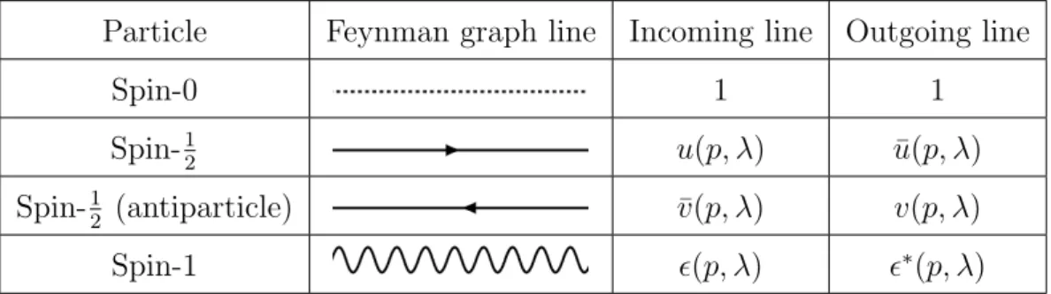
lines represent incoming and outgoing particles. Depending on the spin of a particle there is

a corresponding factor as shown in Table 1.1. Possible types of internal lines, or propagators,

Particle Feynman graph line Incoming line Outgoing line

Spin-0 1 1

Spin- ¹ ₂ u(p, λ) u(p, λ) ¯

Spin- ¹ ₂ (antiparticle) ¯ v(p, λ) v(p, λ)

Spin-1 (p, λ) ^∗ (p, λ)

Table 1.1: Expressions for external lines

Spin-0 −i

Z d ⁴ p (2π) ⁴

1 p ² + m ² − i0

Spin- ¹ ₂ −i

Z d ⁴ p (2π) ⁴

− i/p + m p ² + m ² − i0

Spin-1 (R _ξ gauge) −i

Z d ⁴ p (2π) ⁴

η _µν + (ξ − 1) _p

^p +ξm

^p

p ² + m ² − i0 Table 1.2: Expressions for internal lines (propagators)

and their expressions are listed in Table 1.2, where the term −i0 in the denominator represents small imaginary shift to avoid poles during integration. The situation is a bit more complicated with vertices, since there are many different types of them in the Standard Model. For example, a vertex for the QED interaction γe ⁺ e ⁻ contributes a factor of

− eγ ^µ (2π) ⁴ δ ⁴ (p _a − p _b ) , (1.96) where p _a and p _b are incoming and outgoing 4-momenta respectively, so that the delta-function conserves the total 4-momentum of the system. For all possible vertices of the SM interactions see [5].

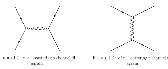
Going back to our example (e ⁺ e ⁻ → e ⁺ e ⁻ ), let us draw the two leading-order diagrams (Figures 1.1 and 1.2) for this process. The time axis conventionally goes from left to right, and while the arrows on the external lines of electrons coincide with the flow of time, those of positrons are often drawn pointing backwards in time (although if we label each line by the particles’ names, we can ignore this convention and draw every arrow on external lines pointing towards future).

So the top-left external line of both diagrams (1.1 and 1.2) represent incoming positron, while

top-right lines represent outgoing positron. Similarly, bottom-left and -right lines stand for

incoming and outgoing electron, respectively. If we are considering only QED, the wiggly line

represents photon. But in the full Standard Model the same diagrams appear with Z boson

propagator as well.

Figure 1.1: e ⁺ e ⁻ scattering s-channel di- agram

Figure 1.2: e ⁺ e ⁻ scattering t-channel di- agram

Putting together the Feynman rules we listed above for the diagram in Figure 1.1, we obtain the S-matrix element (in Feynman-’t Hooft gauge, ξ = 1)

S _ba (s) = −ie ² Z

d ⁴ k(2π) ⁴ δ ⁴ (p ₁ + p ₂ − k)δ ⁴ (k − p ₃ − p ₄ )(¯ v ₁ γ ^µ u ₂ ) η _µν

k ² − i0 (¯ u ₄ γ ^ν v ₃ ) , (1.97) where k is the photon 4-momentum. Then, performing the integration and using (1.81) we find

M _ba (s) = e ² (¯ v ₁ γ ^µ u ₂ ) η _µν

(p ₁ + p ₂ ) ² (¯ u ₄ γ ^ν v ₃ ) , (1.98) called the s-channel amplitude, and the corresponding diagram called the s-channel diagram, because the Mandelstam variable s = −(p ₁ + p ₂ ) ² . Similarly reading off the t-channel diagram in Figure 1.2, we obtain exactly (1.95). Again, the name t-channel follows from the Mandelstam variable t = −(p 1 − p 3 ) ² .

1.1.6 Renormalization

Renormalization is a reparametrization procedure of coupling constants of a theory, with the aim to eliminate the dependence of the physical quantities, like amplitudes, on the (ultraviolet, or UV) cut-off scale Λ. Naively, Λ can be taken arbitrarily large, however, it is inevitable that new physics will appear at some point (e.g. Grand Unification, quantum gravity), and so Λ should be taken as the corresponding scale. When couplings are renormalized they absorb the Λ-dependence of physical quantities, and become functions of the ”running” scale - the scale at which the related physical process takes place. The couplings in the Lagrangian are referred to as bare couplings. The renormalized couplings are sums of the bare couplings and the infinity of loop contributions. If a coupling is small, it, of course, makes every subsequent term less and less significant.

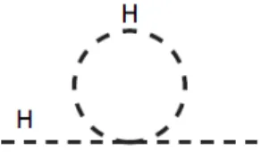
As an example, consider the effective electromagnetic coupling e measured at the scale of the

electron mass m e , say, in a QED scattering process. For a tree-level Feynman diagram in Figure

1.3 (left), there is a one-loop diagram with a fermionic loop, called the self-energy diagram. So,

Figure 1.3

at one-loop order, the aforementioned coupling reads e ² (m _e ) = e ² ₀ − e ⁴ ₀

12π ² log Λ ²

m ² _e

+ O(e ⁶ ₀ ) , (1.99)

where the first term on the RHS comes from the tree-level diagram (Figure 1.3, left), while the second term comes from the one-loop self-energy diagram (Figure 1.3, right).

Next, consider a similar scattering process but with a large momentum transfer p ² m ² _e . The amplitude for this process is proportional to

M ∝ e ² ₀ − e ⁴ ₀ 12π ² log

Λ ² p ² e ^−5/3

+ O(e ⁶ ₀ ) . (1.100)

When substituting (1.99), and replacing e ⁴ ₀ with e ⁴ (m e ) (the difference is of higher order and can be neglected), Λ-dependence is cancelled because the logarithm term from (1.99) enters with the opposite sign.

We can generalize the expression (1.99) for e ² at arbitrary (”running”) scale µ, e ² (µ) = e ² ₀ − e ⁴ ₀

12π ² log Λ ²

µ

+ O(e ⁶ ₀ ) , (1.101)

and, in order to see how e ² runs with µ, substitute e ² ₀ from (1.99). We obtain e ² (µ) = e ² (m _e ) − e ⁴ (m _e )

12π ² log m ² _e

µ

+ O(e ⁶ (m _e )) , (1.102) and further generalize it by differentiating with respect to µ ² to get

µ ² de ² (µ)

µ ² = e ⁴ (m _e )

12π ² + O(e ⁶ (m _e )) . (1.103)

The quantity µ ^{2 de} _µ

^(µ)

≡ β(e) is called the renormalisation group beta function.

The beta functions for the SM interactions (i = 1, 2, 3 for U (1) _Y , SU (2) _L , SU (3) _C respectively) read

β _i (g) = b _i g _i ⁴

12π ² , (1.104)

G ^a _µ (8, 1, 0) W _µ ⁱ (1, 3, 0) B _µ (1, 1, 0)

Table 1.3: SM gauge bosons

with

b ₁ = 41

10 , b ₂ = − 19

6 , b ₃ = −7 , (1.105)

and g _i - coupling constants. Computation of b _i is rather technical, but note that b ₁ is positive and b ₂ , b ₃ are negative, which result in different behaviour of couplings: α ₁ decreases at higher energies while α ₂ and α ₃ increase. This results in asymptotic freedom in QCD, in particular.

The general solution of (1.103), in terms of α _i ≡ g _i ² /4π and with m _e yet again generalized by µ ₀ , reads

α _i ⁻¹ (µ) = α ⁻¹ _i (µ ₀ ) + b _i 3π log

µ ² ₀ µ ²

, (1.106)

and is referred to as Renormalization Group Equations. They define running of the couplings.

1.2 Standard Model particles

The three forces of the Standard Model (SM) - electromagnetic, weak, and strong - are described by a gauge theory based on the combined SU (3) _c × SU(2) _L × U (1) _Y gauge group, where SU(3) _c corresponds to QCD (c for colour), and SU(2) _L × U(1) _Y corresponds to the electroweak interaction. Subscript L stands for ”left”, since only left-chiral fermions transform non-trivially under SU(2) _L . More precisely, they form SU (2)-doublets, while right-chiral fermions are SU (2)- singlets. Subscript Y denotes so-called hypercharge, to distinguish it from the electric charge.

While SU(3) _c symmetry is exact, electroweak symmetry is spontaneously broken as SU (2) _L × U(1) _Y → U (1) _em , where U (1) _em is a gauge group of electromagnetic interaction, the coupling constant of which is the electric charge. U (1) _em symmetry is a combination of U (1) _Y and the U(1) group sitting inside SU (2) _L .

Gauge boson content of the SM consists of 8 SU (3) c gauge bosons - gluons G ^a _µ , transforming as octet under the corresponding gauge group; 3 SU(2) _L (sometimes called ”weak”) gauge bosons W _µ ⁱ , transforming as triplet; and the U(1) _Y gauge boson B _µ . We use indices a, b, c = 1, ..., 8 for SU(3) c group, and i, j, k = 1, 2, 3 for SU(2) L . Transformation properties of the gauge bosons under SU (3) _c × SU(2) _L × U (1) _Y are summarized in Table 1.3. The first number in the parentheses stands for SU(3) _c multiplicity, second one - for SU(2) _L multiplicity, and the last one is hypercharge Y .

Fermionic content consists of ”fundamental” spin-1/2 particles which can be divided into leptons

and quarks. Leptons are defined as fermions that are SU (3) _c singlets, i.e. that don’t participate

in strong interactions. They are: electron e, muon µ, tau lepton τ, and associated neutrinos ν _e , ν _µ , ν _τ . Quarks, on the other hand, are fermions that do carry colour charge and interact strongly. However, unlike leptons, at low energies they are only found in bound colour-neutral states - baryons (combination of 3 quarks) and mesons (combination of quark and anti-quark).

There are six quark ”flavours”: up u, down d, strange s, charm c, top t, and bottom b. Each of them carry one of the three colour charges conventionally denoted r (red), g (green), and b (blue). Quarks and leptons can also be grouped into 3 generations, with each successive generation essentially being just a heavier version of the previous generation with the same quantum numbers. So, the three generations of leptons are e and ν _e , µ and ν _µ , τ and ν _τ . And for quarks - u and d, s and c, t and b. Interestingly, members of each generation of both quarks and leptons differ by one unit of electric charge. For example, e has an electric charge Q(e) = −1, while Q(ν _e ) = 0; similarly Q(u) = +2/3 and Q(d) = −1/3.

In the Standard Model it is convenient to use Weyl or Majorana spinors to represent left- and right-chiral ⁴ components of Dirac spinors, since they transform differently under SU (2) _L . The Dirac spinor of the electron (and its heavier cousins muon and tau) can be decomposed to left and right Weyl spinors as

e = e

e

. (1.107)

Then to translate this into the language of Majorana spinors, we define (in the notation of [5]) E =

e

iσ ₂ e ^∗

, E =

−iσ ₂ e ^∗

e

, (1.108)

where E and E are Majorana spinors containing left and right Weyl spinors respectively, and σ 2 is the second Pauli matrix. Now, using projection operators (see appendix) P L and P R , it is easy to see that

e = P _L E + P _R E . (1.109)

Left-chiral electron (mu, tau) E and the electron (mu, tau) neutrino ν (which has only left-chiral component) form an SU (2) _L doublet L:

L _m = ν

E

m

, (1.110)

where we use the index m = 1, 2, 3 to distinguish between the three generations. E is an SU(2) _L -singlet. For left-chiral quark doublet we have

Q _m = U

D

m

, (1.111)

while the right-chiral singlets are U m and D m . Here U and U stand for up-type quarks u, c, t; D and D stand for down-type quarks d, s, b. Transformation properties of leptons and quarks are summarized in Table 1.4. Bar over a bold number means complex-conjugate representation.

The electric charge is defined simply as a sum Q = T 3 + Y , where T 3 is the eigenvalue of the third SU (2) _L generator called (third component of) isospin.

4

We sometimes refer to left- and right-chiral (Weyl) spinors just as ”left” and ”right” for simplicity.

P _L L _m (1, 2, −1/2) P _R L _m (1, 2, +1/2) P _L E _m (1, 1, +1) P _R E _m (1, 1, −1) P _L Q _m (3, 2, +1/6) P _R Q _m (¯ 3, 2, −1/6) P _L U _m (¯ 3, 1, −2/3) P _R U _m (3, 1, +2/3) P _L D _m (¯ 3, 1, +1/3) P _R D _m (3, 1, −1/3)

Table 1.4: SM fermions

The last missing piece of the Standard Model that has been experimentally confirmed [15] is the Higgs boson - the only ”fundamental” scalar in the SM. It transforms as (1, 2, +1/2) (while it’s conjugate as (1, 2, −1/2)), i.e. as an SU(2) _L -doublet,

φ = φ ⁺

φ ⁰

, (1.112)

with electrically charged component φ ⁺ and neutral component φ ⁰ . Now we are ready to write down the Standard Model Lagrangian,

L = −(D _µ φ) ^† (D ^µ φ) − 1

2 L ¯ _m DL / _m − 1

2 E ¯ _m DE / _m − 1

2 Q ¯ _m DQ / _m − 1

2 U ¯ _m DU / _m

− 1 2

D ¯ m DD / m − 1

4 G ^a _µν G ^aµν − 1

4 W _µν ⁱ W ^iµν − 1

4 B µν B ^µν − g ₃ ² θ 3

64π ² µνρσ G ^aµν G ^aρσ

− g ₂ ² θ ₂

64π ² _µνρσ W ^iµν W ^iρσ − g ₁ ² θ ₁

64π ² _µνρσ B ^µν B ^ρσ − V (φ, φ ^† )

−(y ^e _mn L ¯ _m P _R E _n φ + y _mn ^u Q ¯ _m P _R U _n φ ˜ + y _mn ^d Q ¯ _m P _R D _n φ + h.c.) , (1.113) where ˜ φ ≡ iσ ₂ φ ^∗ ; y ^f _mn , with f = e, u, d, are Yukawa couplings (scalar-spinor), and V (φ, φ ^† ) is the Higgs potential,

V = −µ ² φ ^† φ + λ(φ ^† φ) ² , (1.114)

with real parameters µ and λ satisfying µ ² > 0 (for spontaneous electroweak symmetry break-

ing) and λ > 0 (for stability). The covariant derivatives depend on the objects they act on as

follows:

D _µ φ = ∂ _µ φ − ig ₂ W _µ ⁱ T ⁱ φ − i

2 g ₁ B _µ φ , (1.115)

D _µ L _m = ∂ _µ L _m +

−ig ₂ W _µ ⁱ T ⁱ + i 2 g ₁ B _µ

P _L L _m +

ig ₂ W _µ ⁱ T ^{i ∗} − i 2 g ₁ B _µ

P _L L _m , (1.116) D _µ E _m = ∂ _µ E _m + ig ₁ B _µ P _R E _m − ig ₁ B _µ P _L E _m , (1.117) D _µ Q _m = ∂ _µ Q _m +

−ig ₃ G ^a _µ T ^a − ig ₂ W _µ ⁱ T ⁱ − i 6 g ₁ B _µ

P _L Q _m +

ig ₃ G ^a _µ T ^a∗ + ig ₂ W _µ ⁱ T ^{i ∗} + i 6 g ₁ B _µ

P _R Q _m ,

(1.118)

D _µ U _m = ∂ _µ U _m +

−ig ₃ G ^a _µ T ^a − 2i 3 g ₁ B _µ

P _R U _m +

ig ₃ G ^a _µ T ^a∗ + 2i 3 g ₁ B _µ

P _L U _m , (1.119) D _µ D _m = ∂ _µ D _m +

−ig ₃ G ^a _µ T ^a + i 3 g ₁ B _µ

P _R D _m +

ig ₃ G ^a _µ T ^a∗ − i 3 g ₁ B _µ

P _L D _m , (1.120) where T ^a = λ ^a /2 with Gell-Mann matrices λ ^a , and T ⁱ = σ ⁱ /2 with Pauli matrices σ ⁱ .

The so-called θ-terms (the terms including θ ₁ , θ ₂ , θ ₃ ) are total derivatives, and do not contribute to classical equations of motion. They are non-perturbative (topological) terms, which are important for CP violation ⁵ .

The reason we do not introduce explicit mass terms for gauge bosons and fermions is that it would break gauge invariance. In the following section we introduce a mechanism, which can give masses to the aforementioned particles, via spontaneous symmetry breaking.

1.3 Spontaneous electroweak symmetry breaking

Mass terms for gauge bosons and fermions in the Lagrangian (1.113) are not allowed, as they would break gauge symmetry. But we know experimentally that the weak force is short-ranged (and does not exhibit confinement, unlike QCD), so that it must be mediated by a massive gauge boson. Furthermore, quarks and leptons are also found to be massive. A way to add masses to a theory while keeping the Lagrangian gauge invariant is to break gauge symmetry spontaneously, which means making the vacuum gauge variant by letting a certain field(s) acquire a non-zero vacuum expectation value(s) (VEV). Then in the SM the need for a fundamental scalar arises, because non-zero vev cannot be assigned to spinor and vector fields (that would break Lorentz symmetry.) With that purpose the Higgs complex scalar field, and the Higgs mechanism were introduced, by which certain particles acquire masses while preserving gauge symmetry of the Lagrangian.

We parametrize the Higgs field by choosing the unitary gauge where its upper (charged) com- ponent vanishes, while the lower (neutral) component is real,

5

For more details on topological terms see e.g. [16], or Chapter 11 of [5].

φ = 1

√ 2

0 υ + H

, (1.121)

where υ is the (real constant) vev, and H is the redefined Higgs field with vanishing vev. Then in vacuum we have

hφi = 1

√ 2 0

υ

, (1.122)

The vacuum defined by this configuration has the residual gauge symmetry SU(3) c × U (1) em . We now examine the perturbative spectrum of the theory. After inserting (1.121) into the Lagrangian (1.113) we first consider the term

L ⊃ −(D _µ φ) ^† D ^µ φ = − 1

2 ∂ _µ H∂ ^µ H − 1

4 g ₂ ² (υ + H) ² W _µ ⁺ W ^−µ − 1

8 (g ₁ ² + g ² ₂ )(υ + H) ² Z _µ Z ^µ , (1.123) where W _µ ¹ and W _µ ² combine as

W _µ ^± ≡ 1

√ 2 (W _µ ¹ ∓ iW _µ ² ) (1.124)

with respective electric charges Q = ±1, and masses M _W ≡ M _W

= 1

2 g ₂ υ . (1.125)

Z _µ is another, electrically neutral, combination,

Z _µ ≡ − sin θ _W B _µ + cos θ _W W _µ ³ , (1.126) where θ _W is the Weinberg angle defined as

sin θ _W ≡ g ₂

p g ₁ ² + g ₂ ² , cos θ _W ≡ g ₁

p g ₁ ² + g ² ₂ . (1.127) The mass of Z _µ reads

M _Z = 1 2

q

g ² ₁ + g ² ₂ υ = M _W

cos θ _W , (1.128)

while the orthogonal field, the photon,

A _µ ≡ sin θ _W B _µ + cos θ _W W _µ ³ (1.129) is massless.

The mass of the Higgs field (H) itself comes from the potential V which yields M _H ² = µ ² = 1

2 λυ ² , (1.130)

where the second equality comes from the vacuum condition V ₀ = − 1

2 µ ² υ ² + 1

4 λυ ⁴ = 0 . (1.131)

The fermion mass terms come from Yukawa couplings L ⊃ − υ

√ 2 (y ^e _mn E ¯ _m P _R E _n + y _mn ^u U ¯ _m P _R U _n + y _mn ^d D ¯ _m P _R D _n + h.c.) , (1.132) where the Higgs VEV picks out specific components of left-chiral doublets. In particular this leaves neutrinos massless. One can add right-chiral (or right-handed) neutral heavy leptons by hand to introduce neutrino masses.

The Yukawa mass matrices M ^f = υy ^f / √

2 in general are not diagonal, which they should be if we want to identify mass eigenstates. We can diagonalize them by six unitary matrices V _L ^f and V _R ^f as

M ˜ ^f = υ

√ 2 V _L ^{f †} y ^f V _R ^f , (1.133)

where ˜ M ^f is diagonal. These six unitary matrices are introduced by redefinition of the fermions as

P _L E _m = (V _L ^e ) _mn P _L E _n ⁰ , P _R E _m = (V _R ^e ) _mn P _R E _n ⁰ ,

P _L U _m = (V _L ^u ) _mn P _L U _n ⁰ , P _R U _m = (V _R ^u ) _mn P _R U _n ⁰ , (1.134) P _L D _m = (V _L ^d ) _mn P _L D _n ⁰ , P _R D _m = (V _R ^d ) _mn P _R D ⁰ _n ,

This, in turn, has an interesting effect on the couplings between quarks and W _µ ^± , L ⊃ ig ₂

√ 2 [W _µ ⁺ U ¯ m γ ^µ P L D m + W _µ ⁻ D ¯ m γ ^µ P L U m ] . (1.135)

After the redefinitions ⁶ (1.134) the interaction terms (1.135) become ig ₂

√ 2 [W _µ ⁺ V _mn U ¯ _m ⁰ γ ^µ P _L D ⁰ _n + W _µ ⁻ (V ^† ) _mn D ¯ _m ⁰ γ ^µ P _L U _n ⁰ ] , (1.136) where V ≡ (V _L ^u ) ^† V _L ^d is known as Cabbibo-Kobayashi-Maskawa (CKM) matrix. It is a 3 × 3 unitary matrix responsible for mixing between different generations of quarks.

After adding neutrino masses to the SM, their mass terms undergo similar diagonalization procedure, and the generation-mixing matrix (analogous to CKM) can be defined. It is named Pontecorvo-Maki-Nakagawa-Sakata (PMNS) matrix.

6

For U and D we may use the redefinitions involving only V

, since (1.135) involves only P

projectors.

1.4 Problems of the Standard Model

The Standard Model of particle physics is a remarkably successful theory. It provides an ex- tremely precise working model of particle interactions at presently available energies. However, the story does not end here, as the SM has a number of problems and unanswered questions.

Let us mention some of these problems:

• One crucial thing the SM does not include is gravity. The difficulty arises if one tries to quantise General Relativity, due to the well-known fact that it is non-renormalisable. Of course one may not care about gravitational effects at scales well below the Planckian one (M _P ≡ (8πG) ^−1/2 ∼ 10 ¹⁸ GeV). But without the proper theory of quantum gravity, our picture of the Universe is not complete. There are at least two types of objects out there, to fully understand which, quantum gravity is necessary – black holes and the ”Big Bang” singularity.

• The hierarchy problem. Why is there such an enormous gap between the electroweak scale and the Planck scale? The latter is ∼ 10 ¹⁶ times larger than the former! In the next chapter we are going to show that the hierarchy problem also leads to extreme fine tuning of the Higgs mass parameter.

• Another big questions in the SM is the origin of quark and lepton masses (or Yukawa couplings). In the SM the Yukawa couplings are input parameters, i.e. their values are put by hand. In the same category is the problem of neutrino masses which are absent in the SM. Although there is a possible solution to this problem (see-saw mechanism), it requires the introduction of a new heavy particle.

• Why are there three generations of leptons and quarks? These are basically three copies of the same particles that differ only in their masses.

• Dark energy. From astronomical observations we know that the visible matter constitutes only a fraction of the total energy density of the Universe. The total energy density is dominated by the dark sector which consists of dark energy and dark matter. Dark energy, in the simplest scenario, is identified with cosmological constant which, in turn, is assumed to be the vacuum energy. However, observations show that the cosmological constant (vacuum energy) is 120 orders of magnitude smaller than the expected value in the SM. This is a very large discrepancy!

• Dark matter. The existence of dark matter poses yet another challenge for the SM. Dark matter is made of particles of unknown origin, that do not interact with the SM particles by means other than gravity.

In the next chapter we introduce SUSY and show that it helps resolve some of the men-

tioned problems.