jpxwp_032917r3_upload

高頻度注文板データの統計解析

:

異市場・同一株式価格間の先行遅行関係

(

要約版

)

林 高樹 慶應義塾大学,首都大学東京, CREST JST 2017年4月28日 林 高樹 (慶應義塾大学) 高頻度データによる先行遅行関係分析 2017年4月28日 1 / 21 概要 研究の目的 • 高頻度領域における証券価格間の先行遅行(lead-lag)時間の推定. • 新手法の提案 • 高頻度データによる実証分析. 先行遅行関係の発生要因の理解, 知識発見 先行遅行時間推定の方法論

• Hoffman, Rosenbaum and Yoshida (2013)

• Dobrev and Schaumburg (2015)

• H. and Koike (2016)

実証分析

• 異市場同一銘柄間分析 (Cross-market, single-asset analysis)

• 国内3市場 (東証, Japannext, Chi-X Japan)

• 林 (2015, 2016, 2017)

• 先行遅行時間推定

Hoffmann-Rosenbaum-Yoshida’s method

Hoffmann, Rosenbaum and Yoshida(2013)

• Formulated a lead/lag estimation problem and proposed an estimator

based on H. and Yoshida (2005)’s covariance estimator (“HY estimator”)

• no “synchronization” needed

• Two continuous semimartingales: X, Y

• Shift Ji (interval for Y ) to the left (past) by θ:

J_−θi = (Ti−1 _{− θ, T}i _{− θ]} • θ-shifted HY estimator: Un(θ)_T := ∞ ! i,j=1 Si≤T (∆iX)(∆jY )K_θi,j, (1) where K_θi,j = 1_{Ii_∩Jj

−θ̸=∅}: θ−shifted “HY factor”

林 高樹 (慶應義塾大学) 高頻度データによる先行遅行関係分析 2017年4月28日 3 / 21

HRY’s method

Hoffmann, Rosenbaum and Yoshida(2013)

Assumption: There exists a latent process "Y s.t. Yt = "Yt_−θ∗. θ∗ is an

unknown constant.

• Y is not observed in real time, but is observed with (constant) delay"

θ∗

• θ∗ > 0: X leads Y

• θ∗ < 0: Y leads X

HRY’s method

Hoffmann, Rosenbaum and Yoshida(2013)

HRY(2013)’s proposal:

• “HRY estimator” for the unknown true lag parameter θ∗

#

θHRY := #θn := arg max

θ_∈Gn|U

n_(θ)

T| (2)

where _Gn is a finite grid satisfying certain regularity conditions.

• In the high-frequency setting , #θHRY is consistent for θ∗ (Theorem 1

of Hoffman, et al(13)).

林 高樹 (慶應義塾大学) 高頻度データによる先行遅行関係分析 2017年4月28日 5 / 21

Estimated HRY measures: micro price, TSE vs JNX

time series plot of ˆθ

0 100 200 300 400 500 -0.04 0.02 s8306, tj, y2013-2014 day theta 0 100 200 300 400 500 -0.04 0.02 s8316, tj, y2013-2014 day theta 0 100 200 300 400 500 -0.04 0.02 s8411, tj, y2013-2014 day theta 0 100 200 300 400 500 -0.04 0.02 s8604, tj, y2013-2014 day theta 0 100 200 300 400 500 -0.04 0.02 s8766, tj, y2013-2014 day theta 0 100 200 300 400 500 -0.04 0.02 s8801, tj, y2013-2014 day theta

Figure 1 : Daily HRY measures, Mitsubishi UFJ FG(8306)–Mitsui Real Estate (8801): TSE–JNX.

Alternative approach: Dobrev-Schaumburg (2015)’s method

Estimated HRY measures:

• Unstable

• Affected by microstructure noise

• Sensitive to jumps

An alternative approach by Dobrev and Schaumburg:

• “High-Frequency Cross-Market Trading: Model Free Measurement

and Applications.” Working paper, 2016.

• Utilizes not price changes but timestamps of the trading activities

• Is not (directly) influenced by “microstructure noise” pertaining to

the behavior of the observed, “inefficient” prices

林 高樹 (慶應義塾大学) 高頻度データによる先行遅行関係分析 2017年4月28日 7 / 21

DS’s method

• I_ti = 1 if traded at t; 0 otherwise. t = 0, 1, . . . , N, j = 1, 2.

• regular spacing with ∆ = _NT .

• Objective function to be maximized:

A(h) := 1

A

N_!−h t=1

I_t1I_t+h2

• where A := min$%_tI_t1,%_tI_t2&.

• Modified objective function:

˜

A(h) := A(h)_{− ¯}A

• where ¯A := _2H+11 %H_h=−HA(h).

本研究における相互共起強度関数A(h)の計算: • 約定系列に付随するタイムスタンプ・データではなく, マイクロプラ イスの変化する時点から成るタイムスタンプ・データを使用する. • さらに, マイクロプライスの変化の正負に応じて, タイムスタンプ・ データを, “買い方向,” “売り方向”に2分割して使用する. 相互共起関数 Figure 2 : 相互共起強度関数A(h)の計算例 (みずほFG (8411), 2014年1月14 日). 第2時間帯 (実線) と第6時間帯(破線).

Estimated DS measures: micro price, TSE vs JNX

0 100 200 300 400 500 − 0.002 0.004 0.008 s8306, tse_jnx, y2013−2014 day theta 0 100 200 300 400 500 − 0.002 0.004 0.008 s8316, tse_jnx, y2013−2014 day theta 0 100 200 300 400 500 − 0.002 0.004 0.008 s8411, tse_jnx, y2013−2014 day theta 0 100 200 300 400 500 − 0.002 0.004 0.008 s8604, tse_jnx, y2013−2014 day theta 0 100 200 300 400 500 − 0.002 0.004 0.008 s8766, tse_jnx, y2013−2014 day theta 0 100 200 300 400 500 − 0.002 0.004 0.008 s8801, tse_jnx, y2013−2014 day theta Figure 3 : DS指標の日次推移(実線は買い方向, 破線は売り方向): 三菱UFJ フィナンシャルグループ(8306)–三井不動産 (8801): TSE–JNX. 林 高樹 (慶應義塾大学) 高頻度データによる先行遅行関係分析 2017年4月28日 11 / 21

Summary statistics of estimated DS measures

summary over Period 7/22/14–12/30/14: Micro price, TSE vs JNX

.

Period 1 Period 2 Period 3 20130104–20140110 20140114–20140718 20140722–20141230 code mean stdev mean stdev mean stdev s8306 0.0029 0.0020 0.0027 0.0018 0.0053 0.0010 s8316 0.0034 0.0012 0.0049 0.0066 0.0054 0.0011 s8411 0.0019 0.0090 0.0014 0.0099 0.0039 0.0021 s8604 0.0033 0.0025 0.0029 0.0028 0.0054 0.0018 s8766 0.0035 0.0209 0.0037 0.0102 0.0045 0.0010 s8801 0.0031 0.0276 0.0018 0.0289 0.0044 0.0014 s8802 0.0040 0.0221 0.0037 0.0011 0.0044 0.0009 s9020 0.0036 0.0024 0.0044 0.0071 0.0047 0.0010 s9432 0.0034 0.0014 0.0044 0.0053 0.0049 0.0010 s9433 0.0033 0.0022 0.0047 0.0070 0.0045 0.0010 s9437 0.0041 0.0158 0.0038 0.0014 0.0048 0.0011 s9984 0.0035 0.0011 0.0061 0.0021 0.0059 0.0014 Table 1 : DS指標の要約統計量(単位: 秒): TSE–JNX, 売買・時間帯区別せず. *expressed in seconds. 林 高樹 (慶應義塾大学) 高頻度データによる先行遅行関係分析 2017年4月28日 12 / 21

観察結果の要約

-1

(TSE–ChiX, JNX–ChXの結果については, 論文内の図表を参照.)

フェーズ1期間は結果が安定的でない. 銘柄間の相違はあるが, TSE

ティックサイズ変更前後 (フェーズ1導入前とフェーズ2導入以降)を比

較すると, おおよそ次のように要約可能:

• TSE–JNX, TSE–ChiX: TSEがPTS二市場に対して, 約4ミリ秒先行.

• フェーズ2以降, 特にTSE–JNXは, TSEの先行度増.

• JNX–ChiX: 先行遅行時間の差は1ミリ秒未満(計測限界以下).

• フェーズ2以降, JNX–ChiXは, JNXの先行からChiXの先行へと変化.

林 高樹 (慶應義塾大学) 高頻度データによる先行遅行関係分析 2017年4月28日 13 / 21

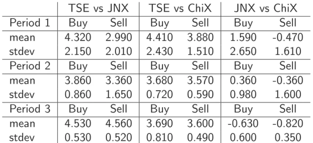
DS

指標の要約統計量

(

売買方向別

)

TSE vs JNX TSE vs ChiX JNX vs ChiX Period 1 Buy Sell Buy Sell Buy Sell mean 4.320 2.990 4.410 3.880 1.590 -0.470 stdev 2.150 2.010 2.430 1.510 2.650 1.610 Period 2 Buy Sell Buy Sell Buy Sell mean 3.860 3.360 3.680 3.570 0.360 -0.360 stdev 0.860 1.650 0.720 0.590 0.980 1.600 Period 3 Buy Sell Buy Sell Buy Sell mean 4.530 4.560 3.690 3.600 -0.630 -0.820 stdev 0.530 0.520 0.810 0.490 0.600 0.350

DS

指標

(

銘柄・期間全体平均

):

売買方向別・時間帯別 0.0025 0.0035 0.0045 t theta 1 2 3 4 5 6 7 8 9 10 Buy: tse_jnx, topix100 prd1 prd2 prd3 0.0030 0.0035 0.0040 0.0045 t theta 1 2 3 4 5 6 7 8 9 10 Buy: tse_chx, topix100 prd1 prd2 prd3 − 0.0010 0.0000 0.0010 t theta 1 2 3 4 5 6 7 8 9 10 Buy: jnx_chx, topix100 prd1 prd2 prd3 0.0025 0.0035 0.0045 t theta 1 2 3 4 5 6 7 8 9 10 Sell: tse_jnx, topix100 prd1 prd2 prd3 0.0030 0.0035 0.0040 0.0045 t theta 1 2 3 4 5 6 7 8 9 10 Sell: tse_chx, topix100 prd1 prd2 prd3 − 0.0010 0.0000 0.0010 t theta 1 2 3 4 5 6 7 8 9 10 Sell: jnx_chx, topix100 prd1 prd2 prd3 Figure 4 : 個別銘柄DS指標の, 各時間帯(横軸)におけるデータ期間内の銘柄全

体平均値(縦軸) (TOPIX100銘柄): TSE–JNX (上段), TSE–ChiX (中段), JNX–ChiX (下段). 買い方向 (左列), 売り方向(右列). 林 高樹 (慶應義塾大学) 高頻度データによる先行遅行関係分析 2017年4月28日 15 / 21 観察結果の要約

-2

全般的な傾向: • フェーズ1導入前, 売買方向間の非対称性大. 特に, 売り側は買い側 に比し先行度がマイナス方向に位置. • フェーズ2導入後, 先行度の売買方向間の差異は縮小. さらに, TSEティックサイズ変更により, • TSE–JNX, TSEの先行度, 特に売り側で大幅増. • TSE–ChiX, TSEの先行度, 特に買い側で減少.

• JNX–ChiX, 買い側はChiXが遅行から先行に変化, 売り側はChiX の

先行度増.

1日内推移:

• 売り方向に“ U 字型 ”. フェーズ1導入前に顕著.

• 買い方向, フェーズ1導入前, 若干の“逆U字 (または逆J字)型.”

Panel regression analysis

• Want to explain how the lead/lag indices are generated in terms of observable

characteristics of the stocks.

• i-th stock, j-th day, t-th time bin

• Covariates (group 1): Ratios between market pairs

• RV rijt = log(RVijtX/RVijtY ): Realized volatility ratio

• N Qrijt = log(N QXijt/N QYijt): # quote revisions ratio

• LT Srijt = log(LT SijtX /LT SijtY ): average lot size ratio

• Sprijt = log(SprijtX /SprYijt): Spread ratio (to mid price) ratio

• QArijt = log(QAXijt/QAYijt): Depth (on Best Ask) ratio.

• QBrijt = log(QBXijt/QBYijt): Depth (on Best Bid) ratio

• Covariates (group 2): Aggregate values of the three markets

• RV agijt: RV of the aggregate market

• RET tsijt: Log return on the TSE

• T V agijt: Total share volume of the aggregate market

• All the variables are standardized.

林 高樹 (慶應義塾大学) 高頻度データによる先行遅行関係分析 2017年4月28日 17 / 21

Panel regression analysis

• Fit a linear mixed effects model to the panel dataset. • yijt = ˆθijt : i-th stock, j-th day, t-th time bin

• T : time-of-the-day effect (t = 1, ..., 10), 6-level factor

• Split the trading hours (300 min.) into ten 30 min. intervals.

• Bin 1: 9-9:30, Bin 2: 9:30-10:00, ..., Bin 10: 14:30-15:00

• Use only Bins 2, 3, 4, 7, 8, 9.

• Dir: Buy direction/ Sell direction, 2-level factor

y _{∼ (1|Code) + (1|Y md)} ! "# $ random ef f ects + _!"#$T 6− level factor + Dir_!"#$ 2− level factor ∗ ⎛ ⎜ ⎝RV r + NQr + LT Sr + SP Rr + QBr + QAr_{! "# $} covariates (group 1) +RV ag + RET ts + T V ag ! "# $ covariates (group 2) ⎞ ⎟ ⎠

Panel regression

• データセットを期間別に3分割し, 市場ペア毎に回帰. • 回帰分析結果. 有意な係数の例: • 正: ボラティリティ比, アスク側デプス比, 等. • 負: スプレッド率比. • 結果の詳細は, 本文を参照. • 林 (2015, 2016)の結果とは必ずしも整合的でない. • 推定結果の頑強性は依然として課題. 林 高樹 (慶應義塾大学) 高頻度データによる先行遅行関係分析 2017年4月28日 19 / 21

Acknowledgement

• Grant-in-Aid for Scientific Research (C), Japan Society for the

Promotion of Science (JSPS), no.16K03601.

• CREST JST Project, Graduate School of Mathematical Sciences,

University of Tokyo.

• Japan Exchange Group, Inc.

• SBI Japannext Co., Ltd

• Chi-X Japan Ltd

References

• 林 (2015). “高頻度注文板データによる2014年東証ティックサイズ 変更の国内株式市場への影響分析.” 証券アナリストジャーナル, 53-4, 29–39. • 林 (2016). “国内高速3株式市場間の注文板形成の先行遅行関係分 析.” ジャフィー・ジャーナル, 128–155.

• Dobrev and Schaumburg. (2015). “High-Frequency Cross-Market

Trading: Model Free Measure- ment and Applications.” Unpublished manuscript.

• H. and Koike (2016). “Wavelet-based methods for high-frequency

lead-lag analysis.” arXiv:1612.01232.

• Hoffmann, Rosenbaum, and Yoshida (2013).“Estimation of the

lead-lag parameter from non-synchronous data,”Bernoulli, 19–2,

426–461.