To give, or not to give; to volunteer, or not to volunteer, that is the question Evidence on Japanese philanthropic behavior revealed by the JGSS-2005 data set

(1)

To give, or not to give; to volunteer, or not to volunteer, that is the question Evidence on Japanese philanthropic behavior revealed by the JGSS-2005 data set

Yoshiho MATSUNAGA Faculty of Business Administration

Osaka University of Commerce

JGSS-2005にみる日本人の寄付行為とボランティア活動

柗永佳甫

大阪商業大学総合経営学部

This paper employs a unique new data set (the JGSS-2005) to test the relationship between giving and volunteering. What factors affect people’s decisions to give and/or to volunteer? Is a giver also a volunteer and vice visa? Research on philanthropic behavior to provide answers to these questions has been overlooked because volunteering is regarded as working for nothing and giving is regarded as a money transfer from one to the other. In short, they do not fit traditional principles of economics. However, philanthropic behavior now receives considerable attention in the literature because several surveys have revealed that the number of people who give time and money is not negligible. While this paper also searches for factors affecting people’s decisions to give and to volunteer, this paper mainly focuses on the direct effect of giving on volunteering and vice visa. The results from our estimation reveal that a volunteer is also a giver, while a giver is not necessarily a volunteer.

Key Words: JGSS, Giving, Volunteering

本稿は、日本人はどのような要因で、寄付あるいはボランティアをするということを決めているのか」ということを、JGSS-2005のデータを用いて明らかにしようとするものである。ボランティアは「無償の労働供給」、寄付は「人から人への単なる資金移転」という視点から、特に経済理論には馴染まないと考えられていたため、これまで慈善活動に関する研究を経済学者が盛んに行うことはなかった。ところが近年、多くの人々が寄付やボランティアを行っていることが明らかとなり、慈善活動に関するより多くの研究がなされるようになった。本稿の目的は、先行研究を参考にしながら、寄付とボランティアの意思決定要因を探りつつ、寄付をする人はボランティアもするのか、ボランティアをする人は寄付もするのか、ということも明らかにしようとするものである。分析の結果、寄付をする人はボランティアもするが、その逆は成り立たないことが明らかとなった。

キーワード：JGSS、寄付、ボランティア

(2)

1. Introduction

Is time more valuable than money? According to USA Today (April, 2005: v133 i2719 p11), many Americans who performed volunteer service maintained that their motivation was to act on their moral values and felt that it is more important to volunteer one's time than to give money to a charitable cause.

Philanthropic behavior such as giving time and money has received little attention as a research agenda for most economists because the decisions regarding whether to volunteer or not and whether to give or not are determined not by people’s economic values but by people’s moral values. As Menchik and Weisbrod (1987) argued, the nature of the supply function of volunteer labor has been overlooked because the wage of volunteer labor is zero. Likewise, giving has been simply considered to be a money transfer from one individual or organization to the other, and from a macroeconomic point of view, people are executing nothing but a zero-sum game.

However, philanthropic behavior now receives considerable attention in the literature because several surveys (e.g. Hodgkinson and Weitzman 1984) have revealed that the number of people who give time and money is not negligible. We now have a significant number of research papers whose research agenda is to investigate the factors affecting people’s decisions to give and to volunteer.

Applying very fundamental concepts of economics to giving and volunteering, such as the opportunity cost of volunteering and the concept of marginal tax rate of giving, several economic theory models of giving and/or volunteering have been developed.

Each previous work has a unique research goal, but what they essentially aim for is to find new factors affecting either the decision to give and/or volunteer or the level of giving and/or volunteering.

These previous papers revealed that researchers basically aimed for finding socio-demographic factors affecting either the decision to give and/or volunteer or the level of giving and/or volunteering depending on the availability of data. Some carried out empirical examinations of theoretic models of giving and/or volunteering that are based on the utility maximization problem within static models (Menchik and Wiesbrod 1987; Smith, Kehoe, Cremer 1995; Freeman 1997; Garcia and Marcuello 2001; Enjolras 2002; Yen 2002; Cappellari and Turati 2004) and dynamic models (Menchik and Wiesbrod 1987; Auten, Sieg, and Clotfelter 2002; Hrung 2004).

Overall, in the previous papers we found inconsistent estimation results of the coefficients of socio-demographic variable. There are several factors that might cause such an inconsistency: (1) the sample size was insufficient; (2) the model for estimation suffered from a specification error; (3) people’s decisions to give and to volunteer vary dramatically in accordance with the locality, because it is likely that philanthropy is heavily dependent upon people’s customs and morality, as USA Today (2005) implied. If factor (1) or factor (3) or both is a feasible cause of the non-robustness of socio-demographic variables, then it is quite conceivable that we observe such inconsistencies in previous papers. If factor (2) is a feasible cause, then it would be sensible to search for a suitable econometric method to estimate equations for giving and/or volunteering. Therefore, we do not explore the cause of such inconsistencies in previous papers, nor do we compare the estimation results in this paper to those in previous papers. Rather, we treat socio-demographic variables simply as control variables in order to perform accurate estimations of the giving model and/or the volunteering model.

Though this paper draws significantly on previous works, we also address unique issues. For

example, do people who volunteer also give and vice visa? If people think that the supply of public

services is the responsibility of the government, then do they increase or reduce the supply of giving

and/or volunteering?

(3)

2. Models and Data 2.1 The econometric model

We consider the following simultaneous probit model (SPM) in order to examine one of our research issues – the question of whether a giver is also a volunteer and vice versa.

 





+ +

=

+ +

=

∗

, ,

2 2 ' 2 2

1 1 ' 1 1

ε β

γ

ε β

γ

X GIVE

VOLR

X VOLR

GIVE

( 1 b ) ) a 1 (

where GIVE = 1 if GIVE

^∗

> 0 , 0 otherwise and

= 1

VOLR if VOLR

^∗

> 0 , 0 otherwise.

This is a conventional simultaneous equations model in the latent, starred structural variables, GIVE

^*

and VOLR

^*

. The observed counterparts are GIVE and VOLR. We assume a bivariate normal distribution with zero means. The variables X

1

and X

2

are independent variables that are assumed to affect the giving equation and the volunteering equation respectively. Following previous papers, we also assume that giving and volunteering would each be functions of the socio-demographic variables such as the level of education, age, and sex and the other variables that may affect the utility maximization problem. Therefore, the explanatory variables X

1

and X

2

contain all the socio-demographic variables available from our data set.

Brown and Lankford (1992) and the Center for Nonprofit Research and Information at Osaka University and UFJ Institute (2005) estimated a giving equation and a volunteering equation assuming that their error terms are correlated with each other or that a giving equation and a volunteering equation are implicitly correlated. Thus, their model is a conventional seemingly unrelated estimator in the latent structural variables, GIVE

^*

and VOLR

^*

, otherwise known as a bivariate probit (BP) model.

However, in our model, GIVE and VOLR appear explicitly in the giving equation and volunteering equation respectively. Consequently, our system of equations (1a) and (1b) is the SPM. This system can be justified because the household or a member of the household will generally change the optimal mix of giving time and money based on economic principles, particularly utility maximization, and the model based on economic principles would have the household or the member of the household explicitly and optimally choosing giving and volunteering. In addition, estimating equation (1a) and (1b) gives us the information that could not be given if we assumed the conventional BP model. That is, whether people who give tend to volunteer and vice versa.

The reduced form and disturbance covariance matrix for the structural variables are

 





+

= +

=

∗

, ,

2 ' 2

1 ' 1

v Z VOLR

v Z GIVE

π π

( 2 b ) ) a 2 (

where 



 



=  Σ

22 21

12 11

σ σ

The matrix form of explanatory variables, Z is all of the exogenous variables including those in

the structural equation and the additional instrumental variables. The identification of (2a) in the

reduced model implies that at least one exogenous variable in X

1

that is not in X

2

has explanatory

power. Likewise, the identification of (2b) implies that at least one exogenous variable in X

2

that is not

in X

1

has explanatory power.

(4)

Table1 Dependent and independent variables

Dependent variables

GIVE =

1 if the respondent made a donation

VOLR =

1 if the respondent participated in volunteer activities

Independent Variables

SEX =

1 if the respondent is male

AGE =

Age at last birthday

SPOUSE =

1 if the respondent is married

REMOTE =

1 if the respondent grew up in a farming or fishing village The level of the respondent's health condition

poor good

0 1 2 3 4

Atheist Not so devoted

Somewhat devoted

Very devoted

0 1 2 3

EDUC =

Respondent's educational attainment

EDUC2 =

Square of the respondent's educational attainment

TPHOUSE =

SCALE1 =

1 if the respondent lives in a middle-sized city

SCALE2 =

1 if the respondent lives in a small city

Individuals and families

OPSRWFY =

⁰ ¹ ² ³ ⁴

COMPEDU =

MEMVLN =

1 if the respondent is a member of volunteer groups

MEMIND =

1 if the respondent is a member of trade associations

MEMCIV =

1 if the respondent is a member of a citizens' movement or consumers' cooperative groups

MEMRL =

1 if the respondent is a member of religious groups

MEMSPT =

1 if the respondent is a member of sports groups

MEMPLT =

1 if the respondent is a member of political associations

Number of child(ren) in compulsory school education

HEALTH =

Education of children

9. 23 million yen or over

6. 8.5 million ~ Less than 12 million

Childcare

Total pre-tax annual income of the household ( including income from stock shares, pensions, and real estate)

RELIG =

3. 2.5 million ~ Less than 4.5 million 4. 4.5 million ~ Less than 6.5 million

Livelihood of the elderly

1 if the respeondent lives in a rental housing 5. 6.5 million ~ Less than 8.5 million

The respondent's opinion of the following statement: "Who do you think should be responsible for dealing with the following social issues? ″

The respondent's opinion of the following statement: "It is the responsibility of the government to reduce the differences in income between families with high incomes and those with low incomes.″

HOUSINC =

7. 12 million ~ Less than 16 million 8. 16 million ~ Less than 23 million 0. None ~ Less than 700,000 yen

1. 700,000 ~ Less than 1.3 million 2. 1.3 million ~ Less than 2.5 million

Medical and nursing care

Governments

(5)

By following Maddala (1983), the two step procedure is to estimate the two reduced forms by the probit MLE (maximum likelihood estimator) method, estimating the two dependent variables using the linear functions, and then to use these linear functions in structural MLEs. The predicted value of GIVE

^*

, that can be obtained by estimating equation (2a) by probit MLEs, is added to the volunteer equation (1b). Likewise, the predicted value of VOLR

^*

, that can be obtained by estimating equation (2b) by probit MLEs is added as the independent variable to equation (1a).

Typical socio-demographic variables given in previous empirical works include SEX, AGE, and SPOUSE, as shown in Table 1. These socio-demographic variables have already been well examined in a significant number of previous works and the results are inconsistent. Therefore, previous papers have revealed that socio-demographic variables are not robust explanatory variables. Thus, this paper regards the socio-demographic variables SEX, AGE, and SPOUSE as control variables in order to capture the accurate effect of the specific explanatory variables corresponding to the research agenda of this paper.

2.2 The data

The data we use in this paper is provided by the JGSS (Japanese General Social Surveys Project) 2005. The General Social Survey (GSS) in the United States served as a model for the JGSS. The GSS is a well-known general social survey that has been conducted repeatedly by the University of Chicago National Opinion Research Center. The JGSS conducts repeated social surveys to study the attitudes and behavior of Japanese people comprehensively. In 1999, the Institute of Regional Studies at the Osaka University of Commerce (the agency conducting the project) was designated as a “key institute on the frontiers of academic projects” by the then Ministry of Education in Japan, recognizing it as an excellent research organization expected to grow in the future; furthermore, it has received support for project promotion. The Institute of Social Science at the University of Tokyo has also acted as a major partner. Basic information about JGSS-2005 in terms of the sampling methods is as follows:

(a) Sample area: Nationwide (e) Number of survey points: 307

(b) Sample population: Men and women 20-89 (f) Number of samples at each survey point: 15 years of age living in Japan (g) Number of respondents contacted: 4,500 (c) Sample size: 4,500 (h) Number of valid responses: 2,023

(d) Sampling method: Two-stage stratified (i) Number of no responses or invalid responses:

random sampling; stratified by regional 2,477

block and population size (j) Response rate: 50.5％

JGSS-2005 was conducted from late August through the beginning of November 2005 and used both interview and placement methods for each respondent. For practical reasons the administrative order (i.e. whether to conduct the face-to-face interview before or after the questionnaire) was determined by the interviewer or administrator depending on the circumstances of each case. In any case the administrative order was recorded for each respondent.

The previous works show that the prices of donating time and that of money are important factors

in people’s decisions of how much time and money to donate. In the case of Japan, the system of tax

deduction is very different from the US. There are only 48 nonprofit organizations that we can obtain

tax deduction. The formula of tax deduction due to donating money to nonprofit organizations is also

quite different from country to country. Tax deductions on donations in the case of political parties are

given by the following formula:

(6)

( )

[ ^min ôf ^30% ^tax ôf ^deduction ^wage încome, ^the âmout ôf ^donating ^money ⁵⁰⁰⁰ ^yen ] ^30%

amount The

×

−

=

whereas tax deductions on donations not in the case of political parties are given by the following formula:

( ^30% ôf ^wage încome, ^the âmout ôf ^donating ^money ) ⁵⁰⁰⁰ ^yen.

min

deduction tax

of amount The

−

=

Therefore, it is not appropriate to define the price of donating money in Japan as in the US case: (1−

Marginal Tax Rate). In addition, according to Center for Nonprofit Research and Information at Osaka University and UFJ Institute (2005), only 3.7% of Japanese people claimed a tax deduction. This tax system does not attract tax payers to donate large amounts of money. Consequently, most charitable donations in Japan are in the form of small contributions collected on the street. Therefore, unlike previous papers using US data, it causes no problem when we estimate models of giving and volunteering ignoring the effect of the price of tax on the decision of giving and volunteering. In addition, according to Yen (2002), the price of giving is absorbed in the constant term in his theoretical and empirical model. Yen (2002) claimed that it is unclear how prices might be distinguished among donation activities.

As far as the price of volunteering (the opportunity cost of volunteering or the wage rate) is concerned, it is possible to calculate it using the JGSS-2005 data. However, this could cause a serious measurement error problem when we estimate equations (1a) and (1b). There are two reasons why this could happen. First, in JGSS-2005 the respondent was asked to state their total hours of volunteering in the last year. However, it is highly unlikely that the respondent would actually be able to precisely remember the total hours of volunteering in the last year. Second, the total annual income of the respondent before tax is categorized in the same way as the total pre-tax annual income of the household (the annual income was categorized into 19 levels). As a result, we cannot obtain a precise wage rate of the respondent or the price of volunteering. Thus, the price of volunteering is not one of the explanatory variables. Hence, the fact that we cannot observe the cross price effects of giving and volunteering seems to represent a shortcoming in the data.

Therefore, we cannot investigate whether the relationship between giving and volunteering is one of substitutes or complements according to the classical economic definition of these terms.

Nonetheless, the coefficient of VOLR and that of GIVE will tell us whether people who give also tend to volunteer and vice versa.

2.3 Our preferred model specification and results from estimations

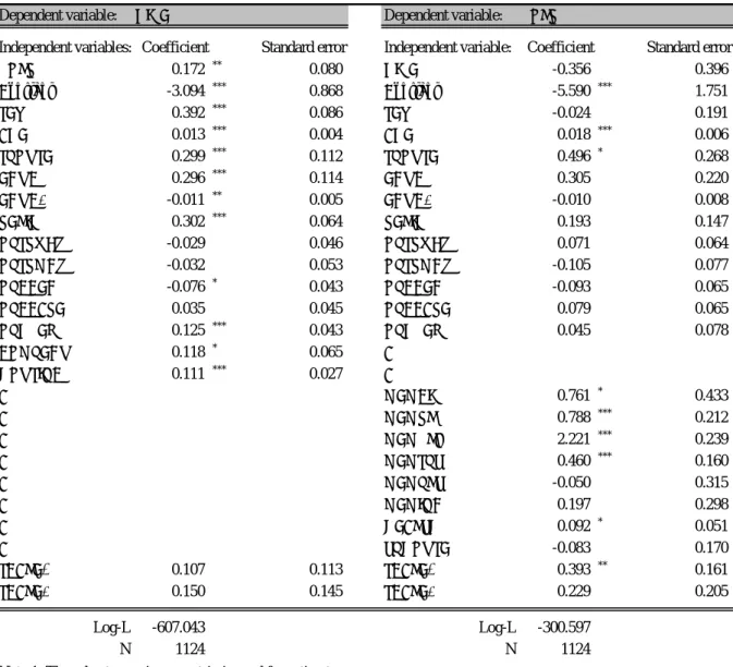
The results from the estimation of equations (1a) and (1b) are given in Table 2.

The rank condition for identifying the volunteering equation (1a) implies that the giving equation must contain at least one exogenous variable with a nonzero coefficient that is excluded from the volunteering equation. The rank condition for identifying the giving equation is simply the mirror image of that of the volunteering equation. Table 2 shows the results from estimating the SPE model.

Table 2 reveals that the rank condition for identifying equation (1a) is satisfied because COMPEDU

and HOUSINC have nonzero coefficients that are excluded from equation (1b). Likewise, the rank

condition for identifying equation (1b) is also satisfied because MEMCIV, MEMRL, MEMVLN,

MEMSPT, and HEALTH and have nonzero coefficients that are excluded from equation (1a).

(7)

Table 2 also reveals that VOLR in equation (1a) has explanatory power (p-value = 0.0308) whereas GIVE in equation (1b) has no explanatory power (p-value = 0.3679).

Table 2 Estimated simultaneous probit equations

Dependent variable: GIVE Dependent variable: VOLR

Independent variables: Coefficient Standard error Independent variable: Coefficient Standard error

VOLR 0.172 ^** 0.080 GIVE -0.356 0.396

Constant -3.094 ^*** 0.868 Constant -5.590 ^*** 1.751

SEX 0.392 ^*** 0.086 SEX -0.024 0.191

AGE 0.013 ^*** 0.004 AGE 0.018 ^*** 0.006

SPOUSE 0.299 ^*** 0.112 SPOUSE 0.496 ^* 0.268

EDUC 0.296 ^*** 0.114 EDUC 0.305 0.220

EDUC2 -0.011 ^** 0.005 EDUC2 -0.010 0.008

RELIG 0.302 ^*** 0.064 RELIG 0.193 0.147

OPSRWFY -0.029 0.046 OPSRWFY 0.071 0.064

OPSRMDY -0.032 0.053 OPSRMDY -0.105 0.077

OPCCED -0.076 ^* 0.043 OPCCED -0.093 0.065

OPCCARE 0.035 0.045 OPCCARE 0.079 0.065

OPGVEQ 0.125 ^*** 0.043 OPGVEQ 0.045 0.078

COMPEDU 0.118 ^* 0.065 -

HOUSINC 0.111 ^*** 0.027 -

- MEMCIV 0.761 ^* 0.433

- MEMRL 0.788 ^*** 0.212

- MEMVLN 2.221 ^*** 0.239

- MEMSPT 0.460 ^*** 0.160

- MEMPLT -0.050 0.315

- MEMIND 0.197 0.298

- HEALTH 0.092 ^* 0.051

- TPHOUSE -0.083 0.170

SCALE1 0.107 0.113 SCALE1 0.393 ^** 0.161

SCALE2 0.150 0.145 SCALE2 0.229 0.205

Log-L -607.043 Log-L -300.597

N 1124 N 1124

Note 1: The robust covariance matrix is used for estimates.

Note 2: ^*, ^**, and ^*** represent 10% significance level, 5% significance level, and 1% siginificance level respectively.

[ ⁼ ¹ ^, ⁼ ⁰ ^| ^, ] ⁼ ^Φ ( ^β ^, ^β ^, ⁻ ^ρ )

Prob GIVE VOLR X

₁

X

₂ _BVN ₁^'

X

₁ ₂^'

X

₂

(3b)

ρ ^(3d)

(8)

where Φ

BVN

is used to depict the cumulative distribution function of the bivariate normal distribution. According to Maddala (1983) and Greene (1998), if the two dependent variables in the modified BP model are jointly determined, then the following equations can be estimated by full information maximum likelihood ignoring the simultaneity in the system.

 





+

=

+ +

=

∗

,

2 2 ' 2

1 1 ' 1 1

ε β

γ X VOLR

X VOLR

GIVE

( 4 ) ) 4a (

b

[ ^, ] ^~ ^bivariate ^normal [ ⁰ ^, ⁰ ^, ¹ ^, ¹ ^, ] ^, ¹ ¹

where ε

₁

ε

₂

ρ − < ρ < ^.

In this system of equations, the correlation between the two structural disturbances (ρ) was allowed to vary freely (The estimation results of the modified BP (MBP) model are not shown). The estimated value was -0.2086 and the t-ratio on this coefficient was -1.149. The null hypothesis thatρ=

0 (against the alternative hypothesis:ρ≠0) cannot be rejected, and therefore, we cannot statistically state that the two structural disturbances are correlated. We also carry out a likelihood ratio (LR) test of H

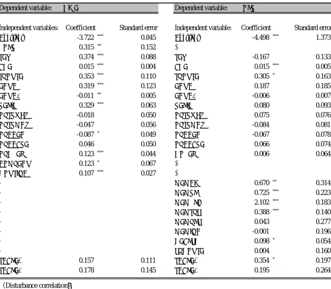
0

:ρ= 0. The test statistic, LR is distributed as chi-squared with one degree of freedom. Since LR = -2[-907.3038-(-907.9678)] = 1.3280 < 3.84, the null hypothesis cannot be rejected. This result is consistent with our t-test result. On the basis of these results, we should re-estimate the MBP model withρ= 0.

Our estimation results of our preferred model shown in Table 3 reveal that it is highly likely that a volunteer is a giver but a giver is not necessarily a volunteer (γ

1

> 0, γ

2

= 0, and ρ= 0). It makes sense because the major charitable donations in Japan are contributions on the street, and being a temporal giver does not lead to being a volunteer. It is highly likely that contributions on the street constitute a one-off form of giving and the amount of giving is relatively small, perhaps around 100 yen (about 80 cents in the US) or so. People make a charitable donation on the street because they hesitate to pass by without giving any money when they run into volunteers who ask for a donation.

However, this type of donation is controlled by donors’ fleeting emotions. Meanwhile, in general people who donate time or engage in volunteer activities belong to volunteer groups or NPOs. Being a member of such organizations occasionally yields a significant number of opportunities to make a charitable donation. Consequently, a volunteer tends to be also a giver. Since this model is considered to be our most preferred model representing the features of our data set, we closely look at the explanatory power of other variables.

Our other research aim relates to whether or not explanatory power can be attributed to the

variables representing people’s opinions regarding the responsibility of the government on social and

economic issues, such as: livelihood of the elderly (OPSRWFY), medical and nursing care of the

elderly (OPSRMDY), education of children (OPCCED), childcare (OPCCARE), and income inequality

(OPGVEQ). The question is, do people increase or decrease the supply of giving and/or volunteering if

they think that the supply of these public services is more the responsibility of the government than the

individual or household. If they think that the supply of public services listed in Table 1 is more the

responsibility of the government than the individual or household, and consequently they decrease the

supply of giving and/or volunteering, then it is conceivable that demand for these public services

should be less than or equal to the supply of these public services by the government. In this case,

there should be no shortage of these public services. However, if they tend to think that the supply of

these public services is more the responsibility of the government than the individual or household and

yet increase the supply of giving and/or volunteering, then it suggests that the demand for these public

services is more than the supply of these public services by the government. People may donate more

(9)

money and/or time to nonprofit organizations so that nonprofit organizations can take on the responsibilities of government as a supplier of these public services. The government failure theory implies that demand heterogeneity is one of the main factors causing the nonprofit sector to expand because nonprofit organizations can supply a variety of public services whereas government supplies only relatively uniform public services.

Table 3 Results from estimation of two probit equations (ρ= 0 is imposed)

Dependent variable: GIVE Dependent variable: VOLR

Independent variables: Coefficient Standard error Independent variable: Coefficient Standard error

Constant -3.722 ^*** 0.845 Constant -4.498 ^*** 1.373

VOLR 0.315 ^** 0.152 -

SEX 0.374 ^*** 0.088 SEX -0.167 0.133

AGE 0.015 ^*** 0.004 AGE 0.015 ^*** 0.005

SPOUSE 0.353 ^*** 0.110 SPOUSE 0.305 ^* 0.163

EDUC 0.319 ^*** 0.123 EDUC 0.187 0.185

EDUC2 -0.011 ^** 0.005 EDUC2 -0.006 0.007

RELIG 0.329 ^*** 0.063 RELIG 0.080 0.093

OPSRWFY -0.018 0.050 OPSRWFY 0.075 0.076

OPSRMDY -0.047 0.056 OPSRMDY -0.084 0.081

OPCCED -0.087 ^* 0.049 OPCCED -0.067 0.078

OPCCARE 0.046 0.050 OPCCARE 0.066 0.074

OPGVEQ 0.123 ^*** 0.044 GOVEQ 0.006 0.064

COMPEDU 0.123 ^* 0.067 -

HOUSINC 0.107 ^*** 0.027 -

- MEMCIV 0.670 ^** 0.314

- MEMRL 0.725 ^*** 0.223

- MEMVLN 2.102 ^*** 0.183

- MEMSPT 0.388 ^*** 0.140

- MEMPLT 0.043 0.277

- MEMIND -0.001 0.196

- HEALTH 0.098 ^* 0.054

- TPHOUSE 0.004 0.160

SCALE1 0.157 0.111 SCALE1 0.354 ^* 0.197

SCALE2 0.178 0.145 SCALE2 0.195 0.264

（Disturbance correlation）

ρ(1,2) 0 (Imposed) Log-L -907.968

NOTE: *, **, and *** represent 10% significance level, 5% significance level, and 1% siginificance level respectively.

Calculated by Limdep 8.0

Table 3 shows that education of children (OPCCED) and income inequality (OPGVEQ) in the giving equation have explanatory power. The coefficient of OPCCED is negative whereas the coefficient of OPGVEQ is positive. Therefore, as people tend to think that the supply of education of children is more the responsibility of the government than of the individual or household, then the probability of giving decreases, thereby implying there exists no shortage of OPCCED . However, if people tend to think that solving income inequality is more the responsibility of government than the individual or household, then the probability of giving increases. Thus, there should be a shortage of public services that is design for solving income inequality.

However, the probability of volunteering is independent of all types of public services listed in

(10)

Table 1. This implies that the shortage or the surplus of these public services does not affect people’s decisions to volunteer or not to volunteer. An important factor affecting people’s decision to volunteer is whether the individual is a member of a citizens’ movement or a consumers’ cooperative group (MEMCIV), religious group (MEMRL), volunteer group (MEMVLN), and sports group (MEMSPT).

The statistically significant coefficients of these variables are all positive. It is conceivable that people who are members of these groups will have more opportunities to volunteer than those who are nonmembers.

There are typical socio-demographic variables, such as SEX, AGE, and SPOUSE, that can be seen in much of the relevant existing literature, that are also included in our model as control variables.

Table 3 shows that the probability of giving is higher for male respondents than female respondents.

The probabilities of both giving and volunteering are higher for elder respondents than younger respondents. This result may be a reflection of the fact that elders tend to have more time for volunteering and more money to give than younger people.

Human capital EDUC and its square, EDUC2, have explanatory powers in the giving equation.

The probability of giving increases at a decreasing rate as the respondent accumulates more human capital. However, the accumulation of human capital has no effect on people’s decisions to volunteer.

RELIG measures the degree of religious belief. The results from our estimation show that the probability of donating money is positively correlated with the degree of faith of the respondent.

However, the degree of religious belief has no effect on the probability of volunteering. This may imply that in Japan giving is considered as a way of showing faith, whereas volunteering is not.

HOUSINC is the pre-tax annual income of the household. The estimation results show that an increase in household income has a positive effect on the probability of giving. As expected, being rich increases the probability of giving.

Health capital HEALTH has positive effect on the probability of volunteering. This result makes sense because if the respondents are not healthy, then it is not likely that they will be able to go out to volunteer.

The proxies for the regional effects are SCALE1 and SCALE2. Only SCALE1 in the volunteering equation has explanatory power, indicating that living in a medium-sized city increases the probability of volunteering. This may imply that a medium-sized city is the preferable size for people to volunteer.

Further research is required in order to investigate this result in detail.

The number of children in compulsory school education COMPEDU increases the probability of giving. A possible reason for this may be that as the number of children in compulsory school education increases, parents will have more opportunities to be asked by the school to make a charitable donation.

2.3 Marginal effects

Before closing section 2, we calculate the marginal effect of the explanatory variable, VOLR on which we have been focusing throughout this paper. The marginal effects of the MBP model are derived by Greene (1996). The conditional mean function in the giving model and the volunteering model is given by

(11)

where Φ is used to depict the cumulative distribution function of the normal distribution. Thus, 1. For a continuous variable, k, that might appear in X

1

and/or X

2

,

[ ] [ ( ) ( ) ( ) ( ) ]

( ) ( ) ( ) ( )

[ ] ^,

,

|

2 1 ' 1 2 ' 2 1

1 ' 1 2 ' 2

1 1 ' 1 2 ' 2 1

1 ' 1 2 ' 2 2

1

k k

X X

X k X

X X GIVE E

β β β

φ γ β

β φ

β β β

γ β

β

Φ

− + + Φ

+

Φ

− Φ + + Φ

Φ

∂ =

∂

(6a)

where φ is used to depict the probability density of the normal distribution.

2. For a binary variable, m, that might appear in X

1

and/or X

2

,

[ ] [ ]

( ) ( ) ( ) ( )

[ ]

( ) ( ) ( ) ( )

[ ] ^| ^| ⁰ ¹ ^.

0 , ,

| 1

, ,

|

1 ' 1 2 ' 2 1

1 ' 1 2 ' 2

1 ' 1 2 ' 2 1

1 ' 1 2 ' 2

2 1 2

1

= Φ

− Φ + + Φ

Φ

−

= Φ

− Φ + + Φ

Φ

=

−

=

m X X

X X

m X X

X X

m X X GIVE E m

X X GIVE E

β β

γ β

β

β β

γ β

β (6b)

3. For an endogenous binary variable, VOLR,

[ ] [ ]

β γ

β + − Φ

Φ

=

−

= (6c)

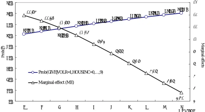
In particular, the marginal effect of VOLR in the giving model can be obtained by applying equation (6c) and its value is 0.0974 (its asymptotic standard error, 0.0427 is computed using the delta method). That is, an increase in the probability of giving is approximately 9.74% for those individuals who volunteer. Note that this marginal effect is computed at the means of the explanatory variables excluding VOLR in the giving model.

80.45%

78.72%

76.87%

74.92%

72.86%

70.69%

68.43%

66.08%

63.65%

61.14%

10.36%

6.48%

7.28%

8.09%

9.65%

8.88%

10.99%

11.54%

11.97%

5.71%

0%

10%

20%

30%

40%

50%

60%

70%

80%

90%

0 1 2 3 4 5 6 7 8 9

5%

6%

7%

8%

9%

10%

11%

12%

13%

Prob(・) Marginal effects

Prob(GIVE|VOLR=1,HOUSINC=0,…,9) Marginal effect (ME)

HOUSINC

Figure 1 The marginal effects of volunteering depending upon household income levels

An interesting observation is that the marginal effect of VOLR in the giving model decreases as the pre-tax annual income of the household, HOUSINC increases (See Figure 1). Each marginal effect in Figure 1 is computed at the means of the explanatory variables excluding VOLR and HOUSINC.

Note that we converted the original 19 categorizations in the JGSS-2005 dataset such that categories 0

and 1 were combined to correspond to level 0, likewise categories 2 and 3 were combined to

(12)

correspond to level 1, and so on up to level 9.

As Figure 1 shows the marginal effect of volunteering on giving tends to be more profound for low income households than that for high income households.

3. Concluding remarks

Analysis of people’s philanthropic activities such as charitable giving and volunteering is in general a challenging research agenda because people’s decisions are closely related to their customs and morality. It is feasible that these activities vary dramatically according to people’s socio-demographic characteristics, by the level of human capital accumulation, by the level of health capital accumulation, and by the locality. The level of religious faith seems also to be an important factor for philanthropic activities. Despite these adverse factors, quite a few researchers have attempted to analyze the factors that determine the level of people’s philanthropic activities. For example some researchers tried to examine the relationship between the level of people’s philanthropic activities and the level of government spending. Abrams and Schmitz (1978) found that such a relationship would imply a crowding out effect, however this finding is not supported by Reece (1979).

Warr (1982) and Roberts (1984) found that increases in government spending on social services encouraged donations. The theoretical framework developed by Schiff (1985) decomposed charitable contributions into an income effect and a substitution effect and showed that government spending need not crowd out charitable contributions and may even encourage giving.

Therefore, as Menchic and Wiesbrod (1987) and Schiff (1985) stated, according to the existing literature the crowding out effects of government spending caused by giving and/or volunteering are ambiguous. Further research is required in order to interpret and investigate this result.

[Acknowledgement]

The Japanese General Social Surveys (JGSS) are designed and carried out at the Institute of Regional Studies at Osaka University of Commerce in collaboration with the Institute of Social Science at the University of Tokyo under the direction of Ichiro TANIOKA, Michio NITTA, Noriko IWAI and Tokio YASUDA. The project is financially assisted by Gakujutsu Frontier Grant from the Japanese Ministry of Education, Culture, Sports, Science and Technology for 1999-2008 academic years, and the datasets are compiled and distributed by SSJ Data Archive, Information Center for Social Science Research on Japan, Institute of Social Science, the University of Tokyo.

[References]

Abrams and Schmitz, 1978, The crowding out effect of governmental transfers on private charitable contributions, Public Choice 33(1):29-39.

Auten, G..E., Sieg H., and Clotfelter, C.T., 2002, Charitable giving, income, and taxes: An analysis of panel data, The American Economic Review Vol.92.No.1:371-381.

Brown, E. and Lankford H., 1992, Gifts of money and gifts of time: Estimating the effects of tax prices and available time, Journal of Public Economics 47:321-341.

Cappellari, L. and Turati, G., 2004, Volunteer labor supply: The role of workers’ motivations, Annals of Public and Cooperative Economics 75(4):619-643.

Center for Nonprofit Research and Information at Osaka University and UFJ Institute, 2005, Giving &

volunteering in Japan 2004, Center for Nonprofit Research and Information.

(13)

Enjolras, B., 2002, Does the commercialization of voluntary organizations ‘crowd out’ voluntary work?, Annals of Public and Cooperative Economics 73(3):375-398.

Freeman, R. B., 1997, Working for nothing: The supply of volunteer labor, Journal of Labor Economics Vol.15(1):s140-166.

Greene W. H., 1996, Marginal effects in the bivariate probit model, Working paper number 96-11, Department of Economics, Stern School of Business, New York University.

Greene W. H., 1998, Gender Economics Courses in liberal arts colleges: Further results, Journal of Economic Education, Volume 29, No.4:291-300.

Hodgkinson, V. and Weitzman, M.,1984, Dimensions of the independent sector: A statistical profile, Independent Sector, Washington D.C..

Hrung, W.B., 2004, After-life consumption and charitable giving, The American Journal of Economics and Sociology Vol.63. No.3:731-745.

Maddala, G.S., 1983, Limited-Dependent and qualitative variables in Econometrics, Cambridge University Press.

Menchik, P.L. and Weisbrod, B.A., 1987, Volunteer labor supply, Journal of Public Economics 32, :159-183.

Reece, W. S., 1979, Charitable contributions: New evidence on household behavior, American Economic Review 69:142-51.

Rivers, D. and Vuong, Q.H., 1988, Limited information estimators and exogeneity tests for simultaneous probit models. Journal of Econometrics 39:347-336.

Roberts, R. D., 1984, A positive model of private charity and public transfers, Journal of Political Economy 92:136-48.

Schiff, J., 1985, Does government spending crowd out charitable contributions?, National Tax Journal 38:535-46.

Smith, V.H., Kehoe, M.R., and Cremer, M.E., 1995, The Private provision of public goods: Altruism and voluntary giving. Journal of Public Economics 58:107-126.