Kernel Dimension Reduction in Regression

Kernel Dimension Reduction in Regression

Kenji Fukumizu

Institute of Statistical Mathematics

4-6-7 Minami-Azabu, Minato-ku, Tokyo 106-8569, Japan

[email protected]

Francis R. Bach

INRIA - WILLOW Project-Team

Laboratoire d’Informatique de l’Ecole Normale Sup´erieure CNRS/ENS/INRIA UMR 8548

45, rue d’Ulm 75230 Paris, France

[email protected]

Michael I. Jordan Department of Statistics

Department of Computer Science and Electrical Engineering University of California, Berkeley, CA 04720, USA

[email protected]

July 23, 2008

Running title. Kernel Dimension Reduction.

AMS 2000 subject classifications. Primary-62H99; secondary-62J02.

Keywords. dimension reduction, regression, positive definite kernel, repro- ducing kernel, consistency.

Acknowledgements. The authors thank the editor and anonymous refer- ees for their helpful comments. The authors also thank Dr. Yoichi Nishiyama for his helpful comments on the uniform convergence of empirical processes.

We would like to acknowledge support from JSPS KAKENHI 15700241,

a research grant from the Inamori Foundation, a Scientific Grant from the

Mitsubishi Foundation, and Grant 0509559 from the National Science Foun-

dation.

Summary

We present a new methodology for sufficient dimension reduction (SDR). Our methodology derives directly from the formulation of SDR in terms of the conditional independence of the covariateX from the response Y, given the projection of X on the central subspace (cf.

[23, 6]). We show that this conditional independence assertion can be characterized in terms of conditional covariance operators on reproduc- ing kernel Hilbert spaces and we show how this characterization leads to an M-estimator for the central subspace. The resulting estimator is shown to be consistent under weak conditions; in particular, we do not have to impose linearity or ellipticity conditions of the kinds that are generally invoked for SDR methods. We also present empirical results showing that the new methodology is competitive in practice.

1 Introduction

The problem of sufficient dimension reduction (SDR) for regression is that of finding a subspace S such that the projection of the covariate vector X onto S captures the statistical dependency of the response Y on X. More formally, let us characterize a dimension-reduction subspace S in terms of the following conditional independence assertion:

Y ⊥ ⊥X | Π

X, (1)

where Π

X denotes the orthogonal projection of X onto S. It is possible to show that under weak conditions the intersection of dimension reduc- tion subspaces is itself a dimension reduction subspace, in which case the intersection is referred to as a central subspace [6, 5]. As suggested in a seminal paper by Li [23], it is of great interest to develop procedures for estimating this subspace, quite apart from any interest in the conditional distribution P (Y | X) or the conditional mean E(Y | X). Once the central subspace is identified, subsequent analysis can attempt to infer a conditional distribution or a regression function using the (low-dimensional) coordinates Π

X.

The line of research on SDR initiated by Li is to be distinguished from the large and heterogeneous collection of methods for dimension reduction in regression in which specific modeling assumptions are imposed on the con- ditional distribution P(Y | X) or the regression E(Y | X). These methods include ordinary least squares, partial least squares, canonical correlation analysis, ACE [4], projection pursuit regression [12], neural networks, and LASSO [29]. These methods can be effective if the modeling assumptions that they embody are met, but if these assumptions do not hold there is no guarantee of finding the central subspace.

Li’s paper not only provided a formulation of SDR as a semiparamet- ric inference problem—with subsequent contributions by Cook and others bringing it to its elegant expression in terms of conditional independence—

but also suggested a specific inferential methodology that has had significant

influence on the ensuing literature. Specifically, Li suggested approaching

the SDR problem as an inverse regression problem. Roughly speaking, the

idea is that if the conditional distribution P (Y | X) varies solely along a sub-

space of the covariate space, then the inverse regression E(X | Y ) should

lie in that same subspace. Moreover, it should be easier to regress X on

Y than vice versa, given that Y is generally low-dimensional (indeed, one-

dimensional in the majority of applications) while X is high-dimensional. Li

[23] proposed a particularly simple instantiation of this idea—known as sliced

inverse regression (SIR)—in which E(X | Y ) is estimated as a constant vec- tor within each slice of the response variable Y , and principal component analysis is used to aggregate these constant vectors into an estimate of the central subspace. The past decade has seen a number of further develop- ments in this vein. Some focus on finding a central subspace [e.g., 9, 10], while others aim at finding a central mean subspace, which is a subspace of the central subspace that is effective only for the regression E[Y |X]. The latter include principal Hessian directions (pHd, [24]) and contour regres- sion [22]. A particular focus of these more recent developments has been the exploitation of second moments within an inverse regression framework.

While the inverse regression perspective has been quite useful, it is not without its drawbacks. In particular, performing a regression of X on Y generally requires making assumptions with respect to the probability dis- tribution of X, assumptions that can be difficult to justify. In particular, most of the inverse regression methods make the assumption of linearity of the conditional mean of the covariate along the central subspace (or make a related assumption for the conditional covariance). These assumptions hold in particular if the distribution of X is elliptic. In practice, however, we do not necessarily expect that the covariate vector will follow an el- liptic distribution, nor is it easy to assess departures from ellipticity in a high-dimensional setting. In general it seems unfortunate to have to impose probabilistic assumptions on X in the setting of a regression methodology.

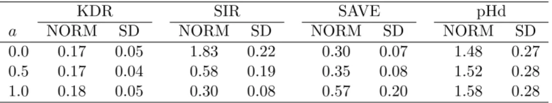
Many of inverse regression methods can also exhibit some additional limitations depending on the specific nature of the response variable Y . In particular, pHd and contour regression are applicable only to a one- dimensional response. Also, if the response variable takes its values in a finite set of p elements, SIR yields a subspace of dimension at most p − 1;

thus, for the important problem of binary classification SIR yields only a one-dimensional subspace. Finally, in the binary classification setting, if the covariance matrices of the two classes are the same, SAVE and pHd also provide only a one-dimensional subspace [7]. The general problem in these cases is that the estimated subspace is smaller than the central subspace.

One approach to tackling these limitations is to incorporate higher-order moments of Y |X [34], but in practice the gains achievable by the use of higher-order moments are limited by robustness issues.

In this paper we present a new methodology for SDR that is rather differ-

ent from the approaches considered in the literature discussed above. Rather

than focusing on a limited set of moments within an inverse regression frame-

work, we focus instead on the criterion of conditional independence in terms

of which the SDR problem is defined. We develop a contrast function for

evaluating subspaces that is minimized precisely when the conditional inde- pendence assertion in Eq. (1) is realized. As befits a criterion that measures departure from conditional independence, our contrast function is not based solely on low-order moments.

Our approach involves the use of conditional covariance operators on reproducing kernel Hilbert spaces (RKHS’s). Our use of RKHS’s is related to their use in nonparametric regression and classification; in particular, the RKHS’s given by some positive definite kernels are Hilbert spaces of smooth functions that are “small” enough to yield computationally-tractable pro- cedures, but are rich enough to capture nonparametric phenomena of inter- est [32], and this computational focus is an important aspect of our work.

On the other hand, whereas in nonparametric regression and classification the role of RKHS’s is to provide basis expansions of regression functions and discriminant functions, in our case the RKHS plays a different role. Our in- terest is not in the functions in the RKHS per se, but rather in conditional covariance operators defined on the RKHS. We show that these operators can be used to measure departures from conditional independence. We also show that these operators can be estimated from data and that these esti- mates are functions of Gram matrices. Thus our approach—which we refer to as kernel dimension reduction (KDR)—involves computing Gram matri- ces from data and optimizing a particular functional of these Gram matrices to yield an estimate of the central subspace.

This approach makes no strong assumptions on either the conditional distribution p

(y | Π

x) or the marginal distribution p

(x). As we show, KDR is consistent as an estimator of the central subspace under weak conditions.

There are alternatives to the inverse regression approach in the litera- ture that have some similarities to KDR. In particular, minimum average variance estimation (MAVE, [33]) is based on nonparametric estimation of the conditional covariance of Y given X, an idea related to KDR. This method explicitly estimates the regressor, however, assuming an additive noise model Y = f (X) + Z, where Z is independent of X. While the purpose of MAVE is to find a central mean subspace, KDR tries to find a central subspace, and does not need to estimate the regressor explicitly.

Other related approaches include methods that estimate the derivative of

the regression function; these are based on the fact that the derivative of

the conditional expectation g(x) = E[y | B

x] with respect to x belongs

to a dimension reduction subspace [27, 18]. The purpose of these methods

is again to extract a central mean subspace; this differs from the central

subspace which is the focus of KDR. The difference is clear, for example, if

we consider the situation in which a direction b in a central subspace sat- isfies E[g

(b

X)] = 0; a condition that occurs if g and the distribution of X exhibit certain symmetries. The direction cannot be found by methods based on the derivative. Also, there has also been some recent work on non- parametric methods for estimation of central subspaces. One such method estimates the central subspace based on an expected log likelihood [35]. This requires, however, an estimate of the joint probability density, and is lim- ited to single-index regression. Finally, Zhu and Zeng [36] have proposed a method for estimating the central subspace based on the Fourier transform.

This method is similar to the KDR method in its use of Hilbert space meth- ods and in its use of a contrast function that can characterize conditional independence under weak assumptions. It differs from KDR, however, in that it requires an estimate of the derivative of the marginal density of the covariate X; in practice this requires assuming a parametric model for the covariate X. In general, we are aware of no practical method that attacks SDR directly by using nonparametric methodology to assess departures from conditional independence.

We presented an earlier kernel dimension reduction method in [13]. The contrast function presented in that paper, however, was not derived as an estimator of a conditional covariance operator, and it was not possible to es- tablish a consistency result for that approach. The contrast function that we present here is derived directly from the conditional covariance perspective;

moreover, it is simpler than the earlier estimator and it is possible to estab- lish consistency for the new formulation. We should note, however, that the empirical performance of the earlier KDR method was shown by Fukumizu et al. [13] to yield a significant improvement on SIR and pHd in the case of non-elliptic data, and these empirical results motivated us to pursue the general approach further.

While KDR has advantages over other SDR methods because of its gen-

erality and its directness in capturing the semiparametric nature of the SDR

problem, it also reposes on a more complex mathematical framework that

presents new theoretical challenges. Thus, while consistency for SIR and

related methods follows from a straightforward appeal to the central limit

theorem (under ellipticity assumptions), more effort is required to study

the statistical behavior of KDR theoretically. This effort is of some general

value, however; in particular, to establish the consistency of KDR we prove

the uniform O(n

) convergence of an empirical process that takes values

in a reproducing kernel Hilbert space. This result, which accords with the

order of uniform convergence of an ordinary real-valued empirical process,

may be of independent theoretical interest.

It should be noted at the outset that we do not attempt to provide distribution theory for KDR in this paper, and in particular we do not address the problem of inferring the dimensionality of the central subspace.

The paper is organized as follows. In Section 2 we show how condi- tional independence can be characterized by cross-covariance operators on an RKHS and use this characterization to derive the KDR method. Section 3 presents numerical examples of the KDR method. We present a consis- tency theorem and its proof in Section 4. Section 5 provides concluding remarks. Some of the details in the proof of consistency are provided in the Appendix.

2 Kernel Dimension Reduction for Regression

The method of kernel dimension reduction is based on a characterization of conditional independence using operators on RKHS’s. We present this characterization in Section 2.1 and show how it yields a population criterion for SDR in Section 2.2. This population criterion is then turned into a finite-sample estimation procedure in Section 2.3.

In this paper, a Hilbert space means a separable Hilbert space, and an operator always means a linear operator. The operator norm of a bounded operator T is denoted by kT k. The null space and the range of an operator T are denoted by N (T ) and R(T ), respectively.

2.1 Characterization of conditional independence

Let (X , B

) and (Y , B

) denote measurable spaces. When the base space is a topological space, the Borel σ-field is always assumed. Let (H

, k

) and (H

, k

) be RKHS’s of functions on X and Y, respectively, with measurable positive definite kernels k

and k

[1]. We consider a random vector (X, Y ) : Ω → X × Y with the law P

. The marginal distribution of X and Y are denoted by P

and P

, respectively. It is always assumed that the positive definite kernels satisfy

E

[k

(X, X)] < ∞ and E

[k

(Y, Y )] < ∞. (2)

Note that any bounded kernels satisfy this assumption. Also, under this

assumption, H

and H

are included in L

(P

) and L

(P

), respectively,

where L

(µ) denotes the Hilbert space of square integrable functions with

respect to the measure µ, and the inclusions J

: H

→ L

(P

) and J

:

H

→ L

(P

) are continuous, because E

[f (X)

] = E

[hf, k

( · , X)i

] ≤

kf k

E

[k

(X, X)] for f ∈ H

.

The cross-covariance operator of (X, Y ) is an operator from H

to H

so that

hg, Σ

fi

= E

£

(f(X) − E

[f(X)])(g(Y ) − E

[g(Y )]) ¤

(3) holds for all f ∈ H

and g ∈ H

[3, 13]. Obviously, Σ

= Σ

, where T

denotes the adjoint of an operator T . If Y is equal to X, the positive self-adjoint operator Σ

is called the covariance operator.

For a random variable X : Ω → X , the mean element m

∈ H

is defined by the element that satisfies

hf, m

i

= E

[f (X)] (4) for all f ∈ H

; that is, m

= J

1, where 1 is the constant function.

The explicit function form of m

is given by m

(u) = hm

, k(·, u)i

= E[k(X, u)]. Using the mean elements, Eq. (3), which characterizes Σ

, can be written as

hg, Σ

f i

= E

[hf, k

(·, X) − m

i

hk

(·, Y ) − m

, gi

].

Let Q

and Q

be the orthogonal projections which map H

onto R(Σ

) and H

onto R(Σ

), respectively. It is known [3, Theorem 1]

that Σ

has a representation of the form

Σ

= Σ

V

Σ

, (5) where V

: H

→ H

is a unique bounded operator such that kV

k ≤ 1 and V

= Q

V

Q

.

A cross-covariance operator on an RKHS can be represented explicitly as an integral operator. For arbitrary ϕ ∈ L

(P

) and y ∈ Y , the integral

G

(y) = Z

X ×Y

k

(y, y)(ϕ(˜ ˜ x) − E

[ϕ(X)])dP

(˜ x, y) ˜ (6) always exists and G

is an element of L

(P

). It is not difficult to see that

S

: L

(P

) → L

(P

), ϕ 7→ G

is a bounded linear operator with kS

k ≤ E

[k

(Y, Y )]. If f is a function in H

, we have for any y ∈ Y

G

(y) = hk

( · , y), Σ

fi

= ¡

Σ

f ¢

(y),

which implies the following proposition:

Proposition 1. The covariance operator Σ

: H

→ H

is the restriction of the integral operator S

to H

. More precisely,

J

Σ

= S

J

.

Conditional variance can be also represented by covariance operators.

Define the conditional covariance operator Σ

by Σ

= Σ

− Σ

V

V

Σ

,

where V

is the bounded operator in Eq. (5). For convenience we some- times write Σ

as

Σ

= Σ

− Σ

Σ

Σ

, which is an abuse of notation, because Σ

may not exist.

The following two propositions provide insights into the meaning of a conditional covariance operator. The former proposition relates the operator to the residual error of regression, and the latter proposition expresses the residual error in terms of the conditional variance.

Proposition 2. For any g ∈ H

, hg, Σ

gi

= inf

f∈HX

E

¯

¯ (g(Y ) − E

[g(Y )]) − (f (X) − E

[f (X)]) ¯

¯

.

Proof. Let Σ

= Σ

V

Σ

be the decomposition in Eq. (5), and define E

(f ) = E

¯

¯ (g(Y ) − E

[g(Y )]) − (f(X) − E

[f (X)]) ¯

¯

. From the equality E

(f ) = kΣ

f k

− 2hV

Σ

g, Σ

f i

+ kΣ

gk

,

replacing Σ

f with an arbitrary φ ∈ H

yields

f∈H

inf

E

(f ) ≥ inf

φ∈HX

© kφk

− 2hV

Σ

g, φi

+ kΣ

gk

ª

= inf

φ∈HX

kφ − V

Σ

gk

+ hg, Σ

gi

= hg, Σ

gi

.

For the opposite inequality, take an arbitrary ε > 0. From the fact

that V

Σ

g ∈ R(Σ

) = R(Σ

), there exists f

∈ H

such that

kΣ

f

− V

Σ

gk

≤ ε. For such f

,

E

(f

) = kΣ

f

k

− 2hV

Σ

g, Σ

f

i

+ kΣ

gk

= kΣ

f

− V

Σ

gk

+ kΣ

gk

− kV

Σ

gk

≤ hg, Σ

gi

+ ε

.

Because ε is arbitrary, we have inf

E

(f ) ≤ hg, Σ

gi

.

Proposition 2 is an analog for operators of a well-known result on co- variance matrices and linear regression: the conditional covariance matrix C

= C

− C

C

C

expresses the residual error of the least square regression problem as b

C

b = min

Ekb

Y − a

Xk

.

To relate the residual error in Proposition 2 to the conditional variance of g(Y ) given X, we make the following mild assumption:

(AS) H

+ R is dense in L

(P

), where H

+ R denotes the direct sum of the RKHS H

and the RKHS R [1].

As seen later in Section 2.2, there are many positive definite kernels that satisfy the assumption (AS). Examples include the Gaussian radial basis function (RBF) kernel k(x, y) = exp(−kx − yk

/σ

) on R

or on a compact subset of R

.

Proposition 3. Under the assumption (AS), hg, Σ

gi

= E

£

Var

[g(Y )|X] ¤

(7) for all g ∈ H

.

Proof. From Proposition 2, we have hg, Σ

gi

= inf

f∈HX

Var[g(Y ) − f(X)]

= inf

f∈HX

n Var

£

E

[g(Y ) − f (X)|X] ¤

+ E

£

Var

[g(Y ) − f (X)|X] ¤o

= inf

f∈HX

Var

£

E

[g(Y )|X] − f (X) ¤

+ E

£

Var

[g(Y )|X] ¤ .

Let ϕ(x) = E

[g(Y )|X = x]. Since ϕ ∈ L

(P

) from Var[ϕ(X)] ≤ Var[g(Y )] < ∞, the assumption (AS) implies that for an arbitrary ε > 0 there exists f ∈ H

and c ∈ R such that h = f +c satisfies kϕ−hk

< ε.

Because Var[ϕ(X) − f (X)] ≤ kϕ − hk

≤ ε

and ε is arbitrary, we have inf

Var

£

E

[g(Y )|X] − f (X) ¤

= 0, which completes the proof.

Proposition 3 improves a result due to Fukumizu et al. [13], Proposition 5, where the much stronger assumption E[g(Y )|X = · ] ∈ H

was imposed.

Propositions 2 and 3 imply that the operator Σ

can be interpreted as capturing the predictive ability for Y of the explanatory variable X.

2.2 Criterion of kernel dimension reduction

Let M (m × n; R) be the set of real-valued m × n matrices. For a natural number d ≤ m, the Stiefel manifold S

(R) is defined by

S

(R) = {B ∈ M (m × d; R) | B

B = I

},

which is the set of all d orthonormal vectors in R

. It is well known that S

(R) is a compact smooth manifold. For B ∈ S

(R), the matrix BB

defines an orthogonal projection of R

onto the d-dimensional subspace spanned by the column vectors of B. Although the Grassmann manifold is often used in the study of sets of subspaces in R

, we find the Stiefel manifold more convenient as it allows us to use matrix notation explicitly.

Hereafter, X is assumed to be either a closed ball D

(r) = {x ∈ R

| kxk ≤ r} or the entire Euclidean space R

; both assumptions satisfy the condition that the projection BB

X is included in X for all B ∈ S

(R).

Let B

⊆ S

(R) denote the subset of matrices whose columns span a dimension reduction subspace; for each B

∈ B

, we have

p

(y|x) = p

0X

(y|B

x), (8)

where p

(y|x) and p

(y|u) are the conditional probability densities of Y given X, and Y given B

X, respectively. The existence and positivity of these conditional probability densities are always assumed hereafter. As we have discussed in Introduction, under conditions given by [6, Section 6.4]

this subset represents the central subspace (under the assumption that d is the minimum dimensionality of the dimension reduction subspaces).

We now turn to the key problem of characterizing the subset B

using conditional covariance operators on reproducing kernel Hilbert spaces. In the following, we assume that k

(z, z) is a positive definite kernel on ˜ Z = D

(r) or R

such that E

[k

(B

X, B

X)] < ∞ for all B ∈ S

(R), and we let k

denote a positive definite kernel on X given by

k

(x, x) = ˜ k

(B

x, B

x), ˜ (9)

for each B ∈ S

(R). The RKHS associated with k

is denoted by H

. Note

that H

= {f : X → R | there exists g ∈ H

such that f (x) = g(B

x)},

where H

is the RKHS given by k

. As seen later in Theorem 4, if X and Y are subsets of Euclidean spaces and Gaussian RBF kernels are used for k

and k

, under some conditions the subset B

is characterized by the set of solutions of an optimization problem:

B

= arg min

B∈S^m_d(R)

Σ

, (10) where Σ

and Σ

denote the (cross-) covariance operators with respect to the kernel k

, and

Σ

= Σ

− Σ

Σ

Σ

.

The minimization in Eq. (10) refers to the minimal operators in the partial order of self-adjoint operators.

We use the trace to evaluate the partial order of self-adjoint operators.

While other possibilities exist (e.g., the determinant), the trace has the advantage of yielding a relatively simple theoretical analysis, which is con- ducted in Section 4. The operator Σ

is trace class for all B ∈ S

(R), since Σ

≤ Σ

and Tr[Σ

] < ∞, which is shown in Section 4.2.

Henceforth the minimization in Eq. (10) should thus be understood as that of minimizing Tr[Σ

].

From Propositions 2 and 3, minimization of Tr[Σ

] is equivalent to the minimization of the sum of the residual errors for the optimal predic- tion of functions of Y using B

X, where the sum is taken over a complete orthonormal system {ξ

}

of H

. Thus, the objective of dimension re- duction is rewritten as

B∈S

min

X

f∈H

min

E ¯ ¯ (ξ

(Y ) − E[ξ

(Y )]) − (f (X) − E[f(X)]) ¯ ¯

. (11) This is intuitively reasonable as a criterion of choosing B , and we will see that this is equivalent to finding the central subspace under some conditions.

We now introduce a class of kernels to characterize conditional indepen- dence. Let (Ω, B) be a measurable space, let (H, k) be an RKHS over Ω with the kernel k measurable and bounded, and let S be the set of all probability measures on (Ω, B). The RKHS H is called characteristic (with respect to B) if the map

S 3 P 7→ m

= E

[k(·, X)] ∈ H (12)

is one-to-one, where m

is the mean element of the random variable with

law P . It is easy to see that H is characteristic if and only if the equality

R f dP = R

f dQ for all f ∈ H means P = Q. We also call a positive definite kernel k characteristic if the associated RKHS is characteristic.

It is known that the Gaussian RBF kernel exp(−kx−yk

/σ

) and the so- called Laplacian kernel exp(−α P

i=1

|x

− y

|) (α > 0) are characteristic on R

or on a compact subset of R

with respect to the Borel σ-field [2, 15, 28].

The following theorem improves Theorem 7 in [13], and is the theoretical basis of kernel dimension reduction. In the following, let P

denote the probability on X induced from P

by the projection BB

: X → X . Theorem 4. Suppose that the closure of the H

in L

(P

) is included in the closure of H

in L

(P

) for any B ∈ S

(R). Then,

Σ

≥ Σ

, (13)

where the inequality refers to the order of self-adjoint operators. If further (H

, P

) and (H

, P

) satisfy (AS) for every B ∈ S

(R) and H

is char- acteristic, the following equivalence holds

Σ

= Σ

⇐⇒ Y ⊥ ⊥X | B

X. (14) Proof. The first assertion is obvious from Proposition 2. For the second assertion, let C be an m×(m −d) matrix whose columns span the orthogonal complement to the subspace spanned by the columns of B, and let (U, V ) = (B

X, C

X) for notational simplicity. By taking the expectation of the well-known relation

Var

[g(Y )|U ] = E

£

Var

[g(Y )|U, V ] ¤

+ Var

£

E

[g(Y )|U, V ] ¤ with respect to V , we have

E

£

Var

[g(Y )|U ] ¤

= E

[Var

[g(Y )|X] ¤ +E

£

Var

£

E

[g(Y )|U, V ] ¤¤

, from which Proposition 3 yields

hg, (Σ

− Σ

)gi

= E

£

Var

£

E

[g(Y )|U, V ] ¤¤

. It follows that the right hand side of the equivalence in Eq. (14) holds if and only if E

[g(Y )|U, V ] does not depend on V almost surely. This is equivalent to

E

[g(Y )|X] = E

[g(Y )|U ]

almost surely. Since H

is characteristic, this means that the conditional

probability of Y given X is reduced to that of Y given U .

The assumption (AS) and the notion of characteristic kernel are closely related. In fact, from the following Proposition, (AS) is satisfied if a charac- teristic kernel is used. Thus, if Y is Euclidean, the choice of Gaussian RBF kernels for k

, k

and k

is sufficient to guarantee the equivalence given by Eq. (14).

Proposition 5. Let (Ω, B) be a measurable space, and (k, H) be a bounded measurable positive definite kernel on Ω and its RKHS. Then, k is charac- teristic if and only if H + R is dense in L

(P ) for any probability measure P on (Ω, B).

Proof. For the proof of “if” part, suppose m

= m

for P 6= Q. Denote the total variation of P − Q by |P − Q|. Since H + R is dense in L

(|P − Q|), for arbitrary ε > 0 and A ∈ B, there exists f ∈ H + R such that R |f − I

|d|P − Q| < ε, where I

is the index function of A. It follows that |(E

[f(X)] − P (A)) − (E

[f (X)] − Q(A))| < ε. Because E

[f (X)] = E

[f (X)] from m

= m

, we have |P (A) − Q(A)| < ε for any ε > 0, which contradicts P 6= Q.

For the opposite direction, suppose H + R is not dense in L

(P ). There is non-zero f ∈ L

(P ) such that R

f dP = 0 and R

f ϕdP = 0 for any ϕ ∈ H. Let c = 1/kfk

, and define two probability measures Q

and Q

by Q

(E) = c R

E

|f |dP and Q

(E) = c R

E

(|f | − f )dP for any measurable set E. By f 6= 0, we have Q

6= Q

, while E

[k(·, X)] − E

[k(·, X)] = c R

f (x)k(·, x)dP (x) = 0, which means k is not characteristic.

2.3 Kernel dimension reduction procedure

We now use the characterization given in Theorem 4 to develop an opti- mization procedure for estimating the central subspace from an empirical sample {(X

, Y

), . . . , (X

, Y

)}. We assume that {(X

, Y

), . . . , (X

, Y

)} is sampled i.i.d. from P

and we assume that there exists B

∈ S

(R) such that p

(y|x) = p

0X

(y|B

x).

We define the empirical cross-covariance operator Σ b

by evaluating the cross-covariance operator at the empirical distribution

P

i=1

δ

δ

. When acting on functions f ∈ H

and g ∈ H

, the operator Σ b

gives the empirical covariance:

hg, Σ b

fi

= 1 n

X

g(Y

)f (X

) − µ 1

n X

g(Y

)

¶µ 1 n

X

f (X

)

¶

.

Also, for B ∈ S

(R), let Σ b

denote the empirical conditional covariance operator:

Σ b

= Σ b

− Σ b

¡ Σ b

+ ε

I ¢

Σ b

. (15) The regularization term ε

I (ε

> 0) is required to enable operator inversion and is thus analogous to Tikhonov regularization [17]. We will see that the regularization term is also needed for consistency.

We now define the KDR estimator B b

as any minimizer of Tr[ Σ b

] on the manifold S

(R); that is, any matrix in S

(R) that minimizes

Tr £

Σ b

− Σ b

¡

Σ b

+ ε

I ¢

Σ b

¤

. (16)

In view of Eq. (11), this is equivalent to minimizing X

a=1

min

f∈H^B_X

· X

i=1

¯ ¯

¯ ¯

½

ξ

(Y

)− 1 n

X

ξ

(Y

)

¾

−

½

f (X

)− 1 n

X

f (X

)

¾¯ ¯

¯ ¯

2

+ε

kf k

¸

over B ∈ S

(R), where {ξ

}

is a complete orthonormal system for H

. The KDR contrast function in Eq. (16) can also be expressed in terms of Gram matrices (given a kernel k, the Gram matrix is the n × n matrix whose entries are the evaluations of the kernel on all pairs of n data points).

Let φ

∈ H

and ψ

∈ H

(1 ≤ i ≤ n) be functions defined by φ

= k

(·, X

) − 1

n X

k

(·, X

), ψ

= k

(·, Y

) − 1 n

X

k

(·, Y

).

Because R( Σ b

) = N ( Σ b

)

and R( Σ b

) = N ( Σ b

)

are spanned by (φ

)

and (ψ

)

, respectively, the trace of Σ b

is equal to that of the matrix representation of Σ b

on the linear hull of (ψ

)

. Note that although the vectors (ψ

)

are over-complete, the trace of the matrix representation with respect to these vectors is equal to the trace of the operator.

For B ∈ S

(R), the centered Gram matrix G

with respect to the kernel k

is defined by

(G

)

= hφ

, φ

i

X

= k

(X

, X

)− 1 n

X

k

(X

, X

)− 1 n

X

k

(X

, X

) + 1

n

X

X

k

(X

, X

),