Estimation of distribution of flow velocity and water elevation in shallow water flow based on the Kalman filter theory
using the finite element method
Takahiko Kurahashi*
Nagaoka University of Technology 1603-1 Kamitomioka, Nagaoka, Niigata, Japan
Email:[email protected]
Shigetoshi Tai
Graduate School of Nagaoka University of Technology 1603-1 Kamitomioka, Nagaoka, Niigata, Japan
Email: [email protected]
Yasuhide Kobayashi Nagaoka University of Technology 1603-1 Kamitomioka, Nagaoka, Niigata, Japan
Email:[email protected]
Taichi Yoshiara
Graduate School of Nagaoka University of Technology 1603-1 Kamitomioka, Nagaoka, Niigata, Japan
Email: [email protected]
Summary
In this study, we present the flow field estimation based on the finite element analysis using the Kalman filter theory. It is known that the Kalman filter theory is one of the methodology that the state value distribution can be estimated by using the system and the observation equations. The influence of the size of the finite element mesh. For the estimated results was investigated in this study.
Keywords: Kalman filter theory, finite element method, shallow water flow
1 Introduction
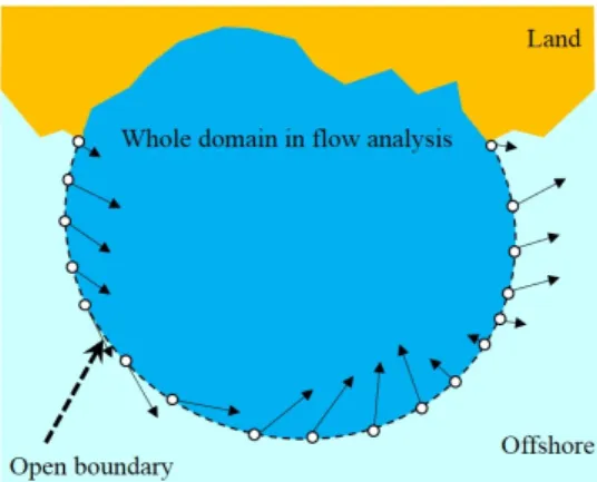
The methodology of the inverse analysis is divided into two approaches, i.e., the deterministic and the stochastic approaches. It is known that the adjoint variable [1] and the direct differentiation methods are one of the deterministic approach, and the Kalman filter theory [2] is one of the stochastic approach. In the Kalman filter theory, the predicted error covariance matrix is expressed by error between the simulated value and the exact value, and the Kalman gain matrix is derived such that the trace norm of the predicted error covariance matrix minimizes. The obtained Kalman gain matrix is used to revise the simulated value by the observed data. The advantage of this theory is to simulate the flow field based on the time history of observation data without considering the open boundary condition such as Figure 1.
In this study, the flow field estimation in the shallow water flow is carried out based on the Kalman filter theory.
The linear shallow water equation is employed as the governing equation, and the finite element method using same order interpolation function for the flow velocity and the water elevation is applied to discretize the governing equation. In addition, the selective lumping method is employed for discretization in time. The purpose of this study is to investigate influence of mesh size for the state values estimated by the Kalman filter theory and the finite element method.
1
Figure 1: Image diagram (Flow analysis considering open boundary condition).
2 Discretization of governing equation in space and time
As for the governing equation, the linear shallow water equation shown in Equations (1) and (2) is employed.
˙
u
i+ g η
,i= 0 (1)
η ˙ +hu
i,i= 0 (2) where u
iindicates the flow velocity for x and y directions, η is water elevation, and g and h mean the gravitational acceleration and standard water depth. In addition, ˙ u
iand η ˙ denote the time derivative of u
iand η , and u
i,iand η
,irepresent the spatial derivative for those variables.
The finite element method using triangular element and the selective lumping method are applied to the discritization in space and time. Consequently, the finite element equation in whole domain is represented as Equation (3).
{ φ
n+1} = [A] { φ
n} (3) where n indicate time step, and vector { φ } consists of the flow velocity u
iand the water elevation η at all nodes. In addition, matrix [A] is derived by the spatial and temporal discretization methods, indicates the superposed finite element matrix in whole domain of target model.
3 State estimation based on Kalman filter theory The revision of the simulated results by the observed value is referred to as "assimilation", and the state value before and after assimilation is expressed by the sign of ( − ) and (+). If the exact state variable vector and the error vector is represented by { φ ˆ } and { p } , the simulated result { φ } , state variable vector, is written as { φ ˆ } + { p } . { φ ˆ } indicates the exact value of the state variable vector { φ } . The discretized governing equation considering the system noise and the observation equation considering the observation noise are shown in Equations (4) and (5).
{ φ ˆ
(−)n+1} = [A] { φ ˆ
(−)n} + [ Γ ] { q
n} (4)
{ z
n+1} = [H] { φ ˆ
n+1} + { r
n+1} (5) Equations (4) and (5) are referred to as the system and the observation equations, respectively. Here, matrices [ Γ ] and [H] are the driving and the observation matrices, { z } denotes the observation vector, and { q } and { r } represent the system noise and the observation noise vectors, respectively.
As the explanation of the computational process of state estimation simulation based on the Kalman filter theory, first of all, the predicted error covariance matrix expressed by error between the simulated value, the estimated value, and the exact value is given by [P]. Next, the Kalman gain matrix [K
1] is derived such that the trace norm of the matrix [P] minimizes. In addition the covariance matrix with respect to the system and the observation errors are expressed by [Q] and [R], respectively, and the computational process of state estimation simulation based on the Kalman filter theory is shown as follows.
In the following computational algorithm, it is assumed that the Kalman gain matrix is time invariant, the computational flow is divided into two parts, i.e., the computation of the Kalman gain matrix (step 1-5) and the computation of the flow field estimation (step 6-8).
1. Input of initial value: Initial condition of the estimated error covariance: [P
(+)] = [ P ˆ
0], Initial condition of state variable: { φ
(+)0} = { φ ˆ
0} , Time steps:imax, Convergence criterion: ε .
2. Computation of predicted error covariance:
[P
(−)] = [A][ P ˆ
(+)][A]
T+ [Γ][Q][Γ]
3. Computation of Kalman gain matrix:
[K
1] = [P
(−)][H]
T([H][P
(−)][H]
T+ [R]
T)
−14. Computation of estimated error covariance:
[P
(+)] = [P
(−)] − [K
1][H][P
(−)]
5. Judgement of convergence by the trace norm of the estimated error covariance matrix after assimilation:
In case of tr[P
(+)] < ε , then go to step 6, In case of tr[P
(+)] > ε , then go to step 2.
6. Update of time step in computation of governing equation:
{ φ
(−)n+1} = [A] { φ
(+)n}
7. Computation of optimal state value after assimilation:
{ φ
(+)n+1} = { φ
(−)n+1} + [K
1]( { z
n+1} − [H] { φ
(−)n+1} ) 8. Judgement of time step: In case of n + 1 = imax, then
stop of computation. In case of n + 1 ̸ = imax, then go to step 6.
4 Numerical experiments
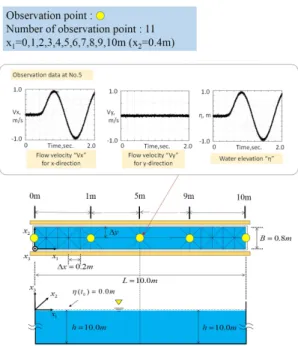
The computational model and location of observation points is shown in Figure 2. In this study, the observed value is expressed by adding white noise and the simulation
2
result. The simulation result is obtained by giving the sine wave, η (t) = sin(2 π t/T ), on the left hand side boundary.
The variable t indicates the time, and the period T in sine wave is set to 0.4 π . The artificial observation data, i.e., summation of the white noise and the simulation result, at x=5m and y=0.4m is also shown in Figure 2.
The computational conditions in the finite element analysis based on the Kalman filter theory is shown in Tab.1. The finite element mesh shown in Figure 3 is employed.
Table 1: Computational conditions Gravitational acceleration g 9.8m/sec
2Lamping parameter e 0.80 Time increment ∆t 0.001sec.
Time steps 2,000
Diagonal components of matrix [Q] 0.010 Diagonal components of matrix [R] 0.001 Convergence criterion ε 10
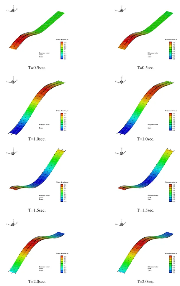
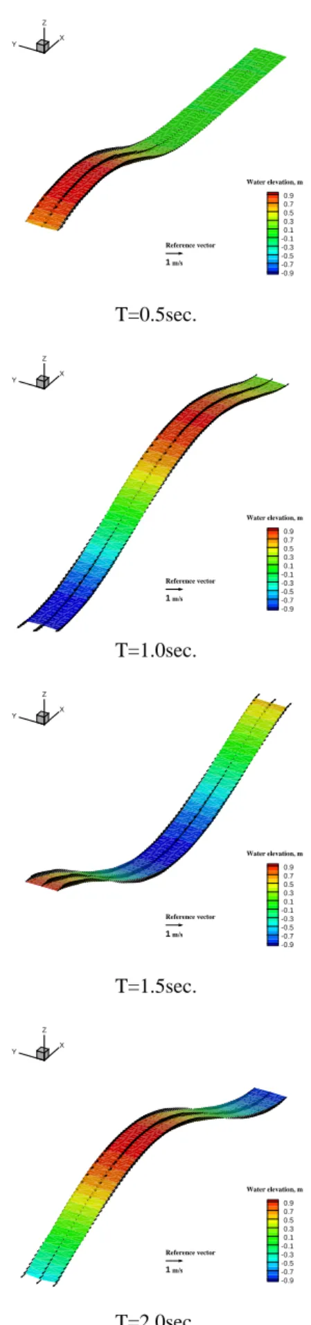
−6As for the computational results, The variation of normalized trace [P] norm is shown in Figure 4. It is seen that the value of normalized trace [P] norm gradually decreases and finally converges. Consequently, the Kalman gain matrix is obtained by the convergence of normalized trace [P] norm. The state value distribution is estimated by the computation of the finite element equation and revision using the Kalman gain matrix and the observed value. The result of the state value distribution by Kalman filter FEM is shown in Figure 5. In addition, the result obtained by the conventional FEM is shown in Figure 6. It is found that similar solutions between the Kalman filter FEM and the conventional FEM are obtained.
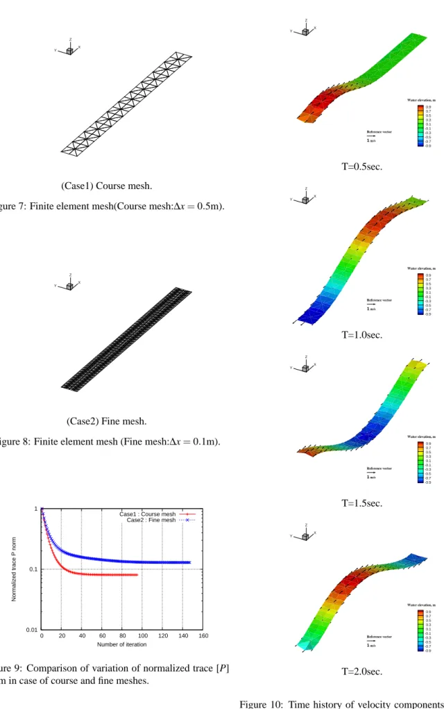
Next, the examinations are carried out by using the course and fine meshes shown in Figures 7 and 8. The variation of normalized trace [P] norm is shown in Figure 9. It is found that normalized trace [P] norm converges as same as the case of the finite element mesh shown in Figure 3. In addition, the result of the state value distribution by Kalman filter FEM are shown in Figures 10 and 11. Even if course and fine meshes are employed, it is found that the obtained solution is similar to the results using the finite element mesh shown in Figure 3.
Figure 2: Computational model, location of observation points and example of artificial observation data at x=5m and y=0.4m.
X Y
Z
Figure 3: Finite element mesh(∆x = 0.5m).
0.01 0.1 1
0 50 100 150 200 250
Normalized trace P norm
Number of iteration Value of trace P norm
Figure 4: Variation of normalized trace [P] norm.
3
X Y
Z
0.9 0.7 0.5 0.3 0.1 -0.1 -0.3 -0.5 -0.7 -0.9 1m/s
Water elevation, m
Reference vector
T=0.5sec.
Y X Z
0.9 0.7 0.5 0.3 0.1 -0.1 -0.3 -0.5 -0.7 -0.9 1m/s
Water elevation, m
Reference vector
T=1.0sec.
X Y
Z
0.9 0.7 0.5 0.3 0.1 -0.1 -0.3 -0.5 -0.7 -0.9 1m/s
Water elevation, m
Reference vector
T=1.5sec.
Y X Z
0.9 0.7 0.5 0.3 0.1 -0.1 -0.3 -0.5 -0.7 -0.9 1m/s
Water elevation, m
Reference vector
T=2.0sec.
Figure 5: Time history of velocity components, u and v, and water elevation η obtained by the Kalman filter FEM using the observation data.
X Y
Z
0.9 0.7 0.5 0.3 0.1 -0.1 -0.3 -0.5 -0.7 -0.9 1m/s
Water elevation, m
Reference vector
T=0.5sec.
Y X Z
0.9 0.7 0.5 0.3 0.1 -0.1 -0.3 -0.5 -0.7 -0.9 1m/s
Water elevation, m
Reference vector
T=1.0sec.
X Y
Z
0.9 0.7 0.5 0.3 0.1 -0.1 -0.3 -0.5 -0.7 -0.9 1m/s
Water elevation, m
Reference vector
T=1.5sec.
Y X Z
0.9 0.7 0.5 0.3 0.1 -0.1 -0.3 -0.5 -0.7 -0.9 1m/s
Water elevation, m
Reference vector
T=2.0sec.
Figure 6: Time history of velocity components, u and v, and water elevation η obtained by the conventional FEM using the boundary conditions.
4
Y X Z
(Case1) Course mesh.
Figure 7: Finite element mesh(Course mesh: ∆ x = 0.5m).
X Y
Z
(Case2) Fine mesh.
Figure 8: Finite element mesh (Fine mesh:∆x = 0.1m).
0.01 0.1 1
0 20 40 60 80 100 120 140 160
Normalized trace P norm
Number of iteration Case1 : Course mesh
Case2 : Fine mesh
Figure 9: Comparison of variation of normalized trace [P]
norm in case of course and fine meshes.
X Y
Z
0.9 0.7 0.5 0.3 0.1 -0.1 -0.3 -0.5 -0.7 -0.9 1m/s
Water elevation, m
Reference vector
T=0.5sec.
Y X Z
0.9 0.7 0.5 0.3 0.1 -0.1 -0.3 -0.5 -0.7 -0.9 1m/s
Water elevation, m
Reference vector
T=1.0sec.
X Y
Z
0.9 0.7 0.5 0.3 0.1 -0.1 -0.3 -0.5 -0.7 -0.9 1m/s
Water elevation, m
Reference vector
T=1.5sec.
Y X Z
0.9 0.7 0.5 0.3 0.1 -0.1 -0.3 -0.5 -0.7 -0.9 1m/s
Water elevation, m
Reference vector
T=2.0sec.
Figure 10: Time history of velocity components, u and v, and water elevation η by the Kalman filter FEM in case of course mesh (∆x=0.5m).
5
X Y
Z
0.9 0.7 0.5 0.3 0.1 -0.1 -0.3 -0.5 -0.7 -0.9 1m/s
Water elevation, m
Reference vector
T=0.5sec.
Y X Z
0.9 0.7 0.5 0.3 0.1 -0.1 -0.3 -0.5 -0.7 -0.9 1m/s
Water elevation, m
Reference vector
T=1.0sec.
X Y
Z
0.9 0.7 0.5 0.3 0.1 -0.1 -0.3 -0.5 -0.7 -0.9 1m/s
Water elevation, m
Reference vector
T=1.5sec.
Y X Z
0.9 0.7 0.5 0.3 0.1 -0.1 -0.3 -0.5 -0.7 -0.9 1m/s
Water elevation, m
Reference vector