Optimal Design of Combined Heat and Power System Using a Genetic Algorithm

(1)

Optimal Design of Combined Heat and Power System Using a Genetic Algorithm

Yoichi Tanaka ¹ , Yoshito Umeda ¹ , Tomoyuki Hiroyasu ² and Mitsunori Miki ²

1. Fundamental Research Department, Toho Gas Co.,Ltd, Tokai, Japan

2. Department of Knowledge Engineering and Computer Sciences, Doshisha University , Kyoto, Japan Abstract: Combined heat and power (CHP) systems generate electric power by means of engine, turbine and fuel cell, and also supply the thermal energy produced through power generation.

Therefore, they are expected to be widespread and contribute to boost total efficiency and save energy.

The optimal design problem of CHP systems is a combinatorial optimization problem involving genera- tors, thermally-activated machines, boilers, chillers and heaters. To solve this problem, the optimal opera- tion of the designed CHP system must be achieved.

In this paper, we formulate the CHP system optimization problem and apply a genetic algorithm with a two stage optimization strategy: the first stage consists of combinatorial optimization, and the second stage consists of operation optimization. Numerical experiments show that the proposed method is effec- tive for the optimal design of CHP systems.

Keywords: Combined heat and power, Genetic algorithm, Engineering Optimization, Optimal design , Optimal operation

1. INTRODUCTION

Combined Heat and Power systems (hereinafter abbre- viated as CHP systems) are power generation systems that are installed in locations requiring electrical power from which both electrical power and thermal energy are obtained at the same time. In recent years, they have been receiving attention because of heightened interests in energy conservation. CHP systems have a generator such as an engine or gas turbine for driving a generator, thermally-activated machines such as an absorption chiller or an exhaust heat boiler that utilizes the exhaust heat from the generator, as well as a supplemental boiler used when the exhaust heat does not produce enough hot water or steam.

Design optimization problems in CHP systems involve the problem optimizing the combination of generators, thermally-activated machines, and supplemental boilers.

However, in order to determine the suitability of a given combination, it is necessary to solve an operation optimi- zation problem for electrical demand, cooling demand, heating demand, and hot water demand, all of which change over time.

Ito and Yokoyama proposed a method where the CHP systems design optimization problem is divided into the operational optimization problem and the system con- figuration design optimization problem, and is then solved in stages. In Ito and Yokoyama’s method, the op- eration optimization problem was solved as a mixed-integer linear programming problem, and the sys- tem configuration design optimization problem was solved by using a gradient method after being simplified [1].

In addition, Fujita et. al pointed out that CHP systems design problem is a complex combinatorial optimization problem, and reported a method to solve the system con- figuration design optimization problem using a genetic algorithm and to solve the operation optimization prob-

lem as a mixed integer linear programming problem us- ing the branch-and-bound method[2].

Although the performance of most machines making up CHP systems is linear, there are some exceptions to this; i.e. machines with efficiencies that drop off dra- matically below a certain load factor. When operation optimization is taken as a mixed-integer linear program- ming problem, handling with this type of exceptional machines is difficult, and this is problematic. For this reason, metaheuristics have been proposed as an ap- proach to the CHP systems operation optimization problem. Ohara et. al proposed a method of using ge- netic algorithms to solve the operation optimization problem for CHP systems made up of fuel cells and heat pumps[3]. However, few examples have been reported of design optimization of CHP systems containing ma- chines with nonlinear performance. In particular, there have been no examples reported in which both the system configuration design and operation are optimized with the nonlinear performance of the machine.

With the CHP systems design problem investigated in this paper, system configuration design was regarded as combination optimization problem to select the optimal machines out of the available candidates, while operation was regarded as a nonlinear optimization problem by ap- proximating machine efficiencies with quadric functions.

By laying out the problem in this way, this CHP systems design optimization method under development makes it possible to flexibly correspond to a wider variety of ma- chines.

A genetic algorithm was used to solve these problems.

It was natural for us to make the attempt adopting the

genetic algorithm with a track record in solving combi-

natorial optimization problems[4] for the optimization of

the configuration making up the CHP systems. More-

over, it would have been conceivable that it is effective to

adopt a genetic algorithm for operation optimization as

(2)

well if taking machine performance to be nonlinear.

Thus, a genetic algorithm specialized for CHP systems design optimization problem was developed, that is able to simultaneously optimize system configuration design and operation, and the effectiveness of this algorithm was verified.

2. FORMULATION OF CHP SYSTEMS OPTIMIZATION PROBLEM

Figure 1 shows the system configuration of the appli- cable CHP systems to be optimized. µ is the energy de- mand that the CHP systems must satisfy, and this is ap- plied as a design parameter.

P is a location where a generator is installed, Q is a lo- cation where a boiler is installed, and R is a location where a thermally-activated machine is installed.

ξ is the total energy input from outside the system into the generators and boilers. υ is the energy required to compensate for insufficient energy input into the ther- mally-activated machines. ζ is the energy amount used to compensate for any differences between energy de- mand and the energy coming out of the CHP systems.

The purpose of this optimization problem is to minimize the total energy input (ξ, υ, and ζ).

D

^I

is the energy input into the generators, D

^O

is the en- ergy output from the generators, E

^I

is the energy input into the boilers, E

^O

is the energy output from the boilers, F

^I

is the energy input into the thermally-activated ma- chines, and F

^O

is the energy output from the ther- mally-activated machines. In addition, Φ is the total energy output from the generators and boilers, while Ω is the total amount of energy out of Φ and υ that does not input into the thermally-activated machines. Ψ is the total energy output of the thermally-activated machines.

The energy amounts described above are vectors made up of 8 components (e

1

, e

2

, e

3

, e

4

, e

5

, e

6

, e

7

, and e

8

).

Here, e

1

is electrical power [kW], e

2

is heat for heating [kW], e

3

is heat for cooling [kW], e

4

is heat for heating water [kW], e

5

is exhaust heat in the form of hot water [kW], e

6

is exhaust heat in the form of gas emissions [kW], e

7

is exhaust heat in the form of steam [kW], and e

8

is the latent heat in municipal gas [kW].

Fig.1 Configuration of CHP system 2.1. Allocation of machines

A generator is chosen from a set G and located on a element of P, where the set G = {g

1

,g

2

,g

3

,…,g

L

} is the set of generators and the set P={P

1

,P

2

,P

3

,…,P

I

} is the set of

the locations of generators. Same kind of generator can be chosen any times.

A boiler is chosen from a set B and located on a ele- ment of Q, where the set B = {b

1

,b

2

,b

3

,…,b

M

} is the set of boilers and the set Q={Q

1

,Q

2

,Q

3

,…,Q

J

} is the set of the locations of boilers. Same kind of boiler can be chosen any times.

A thermally-activated machine is chosen from a set H and located on a element of R, where the set H = {h

1

,h

2

,h

3

,…,h

M

} is the set of thermally-activated ma- chines and the set R={R

1

,R

2

,R

3

,…,R

K

} is the set of the locations of thermally-activated machines. Same kind of thermally-activated machine can be chosen any times.

The 0/1 variables x,y and z are defined as below 1: g

j

is located at P

i

0: g

j

is not located at P

i

1: b

j

is located at Q

i

0: b

j

is not located at Q

i

1: h

j

is located at R

i

0: h

j

is not located at R

i

Only one machine can be located at each location.

On the actual CHP design, there would be the locations where any machine is located. Therefore virtual generator g

1

, which does not have energy input and output, is in- troduced. To locate g

1

at P

i

means that nothing is located at P

i

. Similarly, virtual generator b

1

and virtual ther- mally-activated machine h

1

are introduced to denote that the locations where these machines are located are empty.

When g

1

s are located at every P

i

(i=1,2,3,…,I), the system can not be seen as CHP, therefore the constraint shown below is added.

(4) 2.2. Scheduling of machines 2.2.1. Startup time and stop time

It is not desirable that machines are started and stopped frequently. Therefore, we assume that one startup and stop in the scheduling period, which is a day or a week, is allowed.

Let τ be the last time of the scheduling period. The driving time of the generator located at P

i

(i=1,2,3,…,I) is defined as below.

} :

{

_i^s _i^f

i

t s t s

S = ≤ ≤

s

_i^s

, s

_i^f

∈ { 1 , 2 , 3 ,..., τ }

Where s

^si

and s

^fi

are the startup time and the stop time of the generator respectively.

Similarly, the driving time of the boiler located at Q

i

(i=1,2,3,…,J) is defined as below.

} :

{

_i^s _i^f

i

t t t t

T = ≤ ≤

t

_i^s

, t

_i^f

∈ { 1 , 2 , 3 ,..., τ }

P1

P2

P3

P4

P5

Q1

Q2

Q3

Q4

Q5

R1

R2

R3

R4

R5

DI1t

DI2t

DI3t

DI4t

DI5t

EI1t

EI2t

EI3t

EI4t

EI5t

ξ

t

DO1t

DO2t

DO3t

DO4t

DO5t

EO1t

EO2t

EO3t

EO4t

EO5t

FI1t

FI2t

FI3t

FI4t

FI5t

Φ

t

FO1t

FO2t

FO3t

FO4t

FO5t

Ψ

t

ζ

t

υ

t Ωt

μ

t

En er gy Dem an d

x

ij

= (1)

y

ij

= (2)

z

ij

= (3)

I

x

i i

<

∑

=1 1

(5)

(6)

(3)

Where t

^si

and t

^fi

are the startup time and the stop time of the boiler respectively. The driving time of the ther- mally-activated machine located at R

i

(i=1,2,3,…,K) is defined as below.

} :

{

_i^s _i^f

i

t u t u

U = ≤ ≤

u

_i^s

, u

_i^f

∈ { 1 , 2 , 3 ,..., τ }

Where u

^si

and u

^fi

are the startup time and the stop time of the thermally-activated machine respectively.

Let X,Y and Z denote the 0/1 variables which show the machines are running or not.

They are defined as below.

1 t ∈ S

_i

0 t ∉ S

_i

(i=1,2,…,I,t=1,2,…,τ)

1 t ∈ T

_i

0 t ∉ T

_i

(i=1,2,…,J,t=1,2,…,τ)

1 t ∈ U

_i

0 t ∉ U

_i

(i=1,2,…,K,t=1,2,…,τ) 2.2.2. Load factor

Load factor u,v,w and minimum load factor γ,β,η are defined as below.

u

it

: The load factor of the generator located at P

i

(i=1,2,…,I, t=1,2,…,τ)

v

it

: The load factor of the boiler located at Q

i

(i=1,2,…,J, t=1,2,…τ)

w

it

: The load factor of the thermally-activated machine located at R

i

(i=1,2,…,K, t=1,2,…,τ)

γ

j

: The minimum load factor of the generator g

j

(j=1,2,…,L)

β

j

: The minimum load factor of the boiler b

j

(j=1,2,…,M)

η

j

: The minimum load factor of the thermally-activated machine h

j

(j=1,2,…N)

On the CHP optimal design problem, the design vari- ables are u,v and w. γ,β and η are the constants. u,v and w satisfy the following constraints.

(11) (i=1,2,…,I, t=1,2,…,τ)

(12) (i=1,2,…,J, t=1,2,…,τ)

(11) (i=1,2,…,K, t=1,2,…,τ)

2.3. Evaluation function

ξ

t

is the total fuel input on the time t (t=1,2,…,τ). It is defined as below.

(14)

Φ

t

is the sum of the all generators output and the all boiler output. It is defined as below.

(15)

υ

t

is the compensation for the shortage of the energy for the all thermally-activated machines. It is written as below.

(16)

Where [.]

+

shows the vector which is made by replacing the negative elements of the vector in the brackets with zeros.

Ω

t

is the energy which isn’t put to thermally-activated machines.

(17)

ψ

t

is the sum of output of the total thermally-activated machines.

(18)

The energy which can’t be satisfied by the energy sup- ply from the CHP on the time t (t=1,2,…,τ) is ζ

t

. It is written as below.

(19) The total energy consumption is written as below.

(20) The objective function is defined as below.

(21)

Where a

j

is the j

^th

element of A, and C

j

is the constants.

2.4. Input and output of machines

Input energy and output energy of a machine such as generator, a boiler and a thermally-activated machine are functions of the load factors.

These functions are named as below.

Input energy of generator g

j

: Γ

^Ij

(u) Output energy of generator g

j

: Γ

^Oj

(u)

(j=1,2,…,L), u: load factor Input energy of boiler b

j

: Λ

^Ij

(v)

Output energy of boiler b

j

: Λ

^Oj

(v)

(j=1,2,…,M), v: load factor Input energy of thermally-activated machine h

j

: Θ

^Ij

(w) Output energy of thermally-activated machine h

j

: Θ

^Oj

(w) (j=1,2,…,N), w: load factor

Using these functions, D

^I

,D

^O

,E

^I

,E

^O

,F

^I

and F

^O

are written (7)

it

=

X ⁽⁸⁾

it

=

Y ⁽⁹⁾

it

=

Z ⁽¹⁰⁾

∑

=

≤

L

≤

j

it j

ij

u

x

1

γ 1

∑

=

≤

M

≤

j

it j

ij

v

y

1

β 1

∑

=

≤

N

≤

j

it j

ij

w

z

1

η 1

∑ ∑

= =

+

=

^I

i

J i

I it I

it

t

D E

1 1

ξ

∑ ∑

= =

+

= Φ

^I

i

J i

O it O

it

t

D E

1 1

=



+



 



 − Φ

= ∑

^K

i t

I it

t

F

1

υ

∑

=

− + Φ

=

Ω

^K

i I it t

t

F

1

υ

∑

=

= Ψ

^K

i O it

t

F

1

[ ⁻ ^Ψ ⁻ ^Ω ]

₊

=

_t _t _t

t

µ

ζ

( )

∑

=

+ +

= ^τ ξ υ ζ

1 t

t t

A

t

∑

=

⁸

1

j j j

EV

C a

V

(4)

as below.

if X

it

= 1

0 if X

it

= 0

if X

it

= 1

0 if X

it

= 0

if Y

it

= 1

0 if Y

it

= 0

if Y

it

= 1

0 if Y

it

= 0

if Z

it

= 1

0 if Z

it

= 0

if Z

it

= 1

0 if Z

it

= 0

2.5. Evaluation function and design variables

In this problem, design variables are x,y,z which denote the allocation, and s

^s

,s

^f

,t

^s

,t

^f

,u

^s

,u

^f

which denote the startup and stop, and u,v,w which denote the load factors of the machines. And other variables are dependent variable.

The evaluation function is the equation 21. The aim of this problem is to search the design variables with which the evaluation function takes the minimum value.

3. GENETIC ALGORITHM THAT WAS APPLIED The CHP systems design optimization problem set out in this paper has non-linear evaluation function with a large number of design variables with discrete values makes it difficult to find the strict optimum.

For this reason, we attempted to use a genetic algo- rithm, which is a versatile optimization method, to solve this problem.

3.1. Two-state genetic algorithm

If all the design variables are handled in the same way and simply lined up to create the gene code, the cross- overs would destroy the relationship between machine load factor, startup times, start times, and machine types, which prevents the effective use of the genetic algorithm.

To overcome this problem, the 2-stage algorithm de-

scribed below was devised.

3.1.1. Gene code

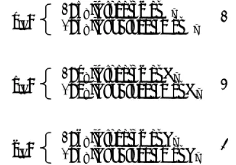
The concept of the gene code used in this Two-stage genetic algorithm is shown in Figure 2. The variables x, y, and z, which express equipment installation, together with the variables s

^s

, s

^f

, t

^s

, t

^f

, u

^s

, and u

^f

, which express start and shutdown times for each equipment, as the inte- ger design variables.

The variables u, v, and w express load factors and are the real number design variables.

In this code, the rows correspond to the installation locations of the equipment. The 1st row shows the val- ues indicating the installed equipment and the 2nd row shows the startup times. The 3rd row shows the end time, while the 4th row and below indicate the load fac- tors at each time value.

Figure 3 shows a specific example of installation lo- cation Pi for design variables layout on the genetic code.

The characteristics of this code are as follows:

(1) For each equipment, the equipment type, startup time, end time, and load factor are one set.

(2) The variables are divided into integer design vari- ables and real number design variables, and optimiza- tion is executed alternating between the two sets as shown in Figure 4.

Fig.2 Structure of genetic code

Fig.3 Genetic code of one equipment

Fig.4 Optimization execution

○◎◎□□□□□□□□□□□□

・・・

○◎◎□□□□□□□□□□□□

・

○◎◎□□□□□□□□□□□□

Genetic Code of One individual

Load factor

Integer

Design Variable Real number Design Variable

P

1

R

5

P

2

P

3

Q

1

Q

2

・・・

R

4

・・・

Start time End time Equipment

Index Code

Time: 1 2 3

Eq ui pm en t Loca tio n :

4 ・・・・

P

i

○◎◎□□□□□□□□□□□□

g

j

when X

ij

=1

s

si

s

fi

u

i1

u

i2

u

i3

u

i4

u

i5

u

i6

・・・・・

Optimization of

Integer Design Variables Optimization of

Real Number Design Variables executed

alternately

・・・・・・

∑

= L

Γ

j

ij I j

ij

u

x

1

)

D

^Iit

= ( (22)

∑

= L

Γ

j

ij O j

ij

u

x

1

)

D

^Oit

= ( (23)

∑

= M

Λ

j

ij I

j

ij

v

y

1

)

E

^Iit

= ( (24)

∑

= M

Λ

j

ij O

j

ij

v

y

1

)

E

^Oit

= ( (25)

∑

= N

Θ

j

ij I j

ij

w

z

1

)

F

^Iit

= ( (26)

∑

= N

Θ

j

ij O

j

ij

w

z

1

)

F

^Oit

= ( (27)

(5)

3.1.2. Mutations

Mutations are introduced as a certain probability of changes to the integer design variables and real number design variables. The integer design variables are sub- jected to mutations during integer design variable opti- mization, while the real number design variables are sub- jected to mutations during real number design variable optimization. The change values are plausible values for each design variable.

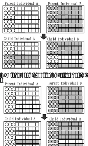
3.1.3. Crossovers

During integer design variable optimization, two ran- domly selected rows are switched as shown in Figure 5.

During real number design variable optimization, only the real number design variables are switched at random as shown in Figure 6.

Fig.5 Crossover on integer design variables optimization stage

Fig.6 Crossover on real number variables optimization stage

3.1.4. Penalties

Those individuals not satisfying the equation (4) have the maximum value of energy consumption amount ap- plied so that they are not selected.

3.1.5. Design of distributed genetic algorithm

A distributed genetic algorithm[5] was adopted as the basic algorithm.

The best individual was chosen using a tournament se- lection. In addition, a bit conversion was not used for the encoding method. Instead, the integer values were used for the integer design variables, while real number values were used for the real number design variables.

Here, the “int” type variables were used for the integer values and “double” type variables were used for the real number values (effective digit: 15 decimal digits).

For both integer design variable optimization and for real number design variable optimization, during one op- timization operation, the selection of fit individuals is carried out on all of the individuals, followed by cross- over on the selected individuals, which is followed by mutations on each of the individuals generated during the crossover step. Both integer design variable optimiza- tion and real number design variable optimization are carried out continuously in the same way until they reach the prescribed final number of generations, when a switch is carried out to another method.

4. PARAMETERS FOR NUMERICAL EXPERIMENT

4.1. Types of machines

In this numerical experiment, the generators were se- lected from those shown in Table 1, the boilers were se- lected from those shown in Table 2, and the ther- mally-activated machines were selected from those shown in Table 3.

Parent Individual A Parent Individual B

Child Individual A Child Individual B

Parent Individual A Parent Individual B

Child Individual A Child Individual B

Table 1. Set of generators G Generator

type Capacity

[kW] Exhaust heat type g

1

No generator

g

2

Gas engine 6 Hot water g

3

Gas engine 25 Hot water g

4

Gas engine 110 Hot water g

5

Gas engine 200 Hot water g

6

Gas engine 350 Hot water g

7

Gas engine 740 Hot water

g

8

Gas turbine 27 Steam

g

9

Gas turbine

27 Exhaust gas

g

10

Gas turbine 60 Steam

g

11

Gas turbine

60 Exhaust gas Table 2. Set of boilers B Boiler type Capacity

[kW]

b

1

No boiler b

2

Steam boiler 60 b

3

Hot water

boiler 60

b

4

Steam boiler 470 b

5

Hot water

boiler 470

b

6

Steam boiler 1250 b

7

Hot water

boiler 1250

(6)

4.2. Machine efficiency

The functions for the energy output of the machines (Γ

^O

, Λ

^O

, and Θ

^O

), the energy input into the machines (Γ

^I

, Λ

^I

, and Θ

^I

) were decided as follows.

The power output from the generators is obtained by multiplying the rated power generation output by the load factor. The input of municipal gas is obtained by divid- ing the power generation output by the power generation efficiency. Exhaust heat output is obtained by multi- plying the input of municipal gas by the exhaust heat col- lection efficiency. The power generation efficiencies of various generators are shown in Figure 7, while the ex- haust heat recovery efficiencies of various generators are shown in Figure 8. The relationship between the effi- ciency and load factor was approximated as a quadratic function and used.

The calculations were performed assuming a fixed ef- ficiency for the boilers and thermally-activated machines.

Fig.8 Heat recovery efficiency 4.3. Energy demand

In this numerical experiment, the final operation time τ

= 24, and energy demand µ

t

(t = 1, 2, 3, …24) was set out as shown in Figure 9. Of the elements for µ

t

, every element other than e

1

(electrical power), e

3

(cooling), e

4

(hot water) were set to zero for all time values.

Fig.9 Energy demand

4.4. Weighting constants of consumed energy

The energy utilization weighting constants C

j

for evaluation function (21) (j = 1, 2, …,8) are as follows:

C

1

=2.86, C

2

=0.952, C

3

=0.952, C

4

=1.25, C

5

=1.25, C

6

=1.0, C

7

=1.25, C

8

= 1.0.

These values are set out from the standpoint of how much primary energy is required to generate a unit amount of the required energy.

4.5. Parameters for genetic algorithm

The parameters for the genetic algorithm are shown in Table 4.

5. RESULTS OF NUMERICAL EXPERIMENT 5.1. Trial Results

A summary of all 50 trials is shown in Figure 10. The evaluation values in the figure are values obtained by equation (21) divided by τ = 24, and its physical meaning is an average energy input. The best, median, and worst value shown in the figure indicate the best, median, and worst values in the 50 trials in each generation. The solid line in the figure is the median value.

The average energy input without a CHP systems is 1295kW, and in each of the test runs, a better solution Table 3. Set of thermally-activated machines

H Thermally-activated

machine type Capacity

[kW] Exhaust heat type

h

1

No machine

h

2

Absorption refrigerator 150 Hot water h

3

Absorption refrigerator 300 Hot water h

4

Absorption refrigerator 450 Hot water h

5

Absorption refrigerator 150 Steam h

6

Absorption refrigerator 300 Steam h

7

Absorption refrigerator 450 Steam h

8

Absorption refrigerator 150 Exhaust gas h

9

Absorption refrigerator 300 Exhaust gas h

10

Absorption refrigerator 450 Exhaust gas

g

11

Heater 500 Hot water

h

12

Heater 500 Steam

h

13

Hot water boiler 500 Hot water h

14

Hot water boiler 500 Exhaust gas

h

15

Hot water boiler 500 Steam

0.2 0.25 0.3 0.35 0.4 0.45

50% 60% 70% 80% 90% 100%

Load Factor

P ow er C oef fic ien t

g2 g3 g4 g5 g6 g7 g8 g9 g10 g11

0.3 0.35 0.4 0.45 0.5 0.55 0.6 0.65

50% 60% 70% 80% 90% 100%

Load Factor

H e a t Re co v er y E ff ici ency

g2 g3 g4 g5 g6 g7 g8 g9 g10 g11

Fig.7 Power generation coefficient

0 100 200 300 400 500 600 700 800 900

1 3 5 7 9 11 13 15 17 19 21 23 Time

Demand [kW]

Electric Power Demand Cooling Demand Hot Water Demand

(7)

than not having CHP systems was selected before 50 generations.

Fig. 10 Transition of evaluation value 5.2. Validity of the solution obtained

Table 5 shows the selected machines. Figure 11 shows the output of the power generation, and Figure 12 shows the exhaust heat utilization status. CHP systems have higher efficiencies if power is generated from the generators when there is no surplus in both power output and exhaust heat output. The solution obtained from the genetic algorithm also had a minimal surplus of exhaust heat, which is a characteristic of high-efficiency CHP systems.

In actual systems, the boiler is installed as a supple- mental role. However, the use of boilers is disadvanta- geous from the standpoint of energy efficiency. Boilers and generators are what produce the energy used by ther- mally-activated machines, and generators output power in addition to the exhaust heat output, which makes it possi- ble to reduce the electrical power element of ζ. Because of this significant effect, if there is a boiler output, it is more efficient to install a generator that is able to produce the same amount of exhaust heat.

In the numerical experiment carried out for this paper, there were no boilers being installed at al and this is a valid result.

Table 4. Parameters of genetic algorithm

item value

Trials number 50

Number of islands 20

Migration rate 0.5

Migration interval 5

Population size 10

Number of generations 500 Number of generations(integer

design variables optimization) 30 Number of generations(real design

variables optimization 60

Tournament size 4

Crossover rate 1.0

Mutation rate(integer design vari-

ables optimization) 0.0222 Mutation rate(real design vari-

ables optimization) 0.002778

1000 1100 1200 1300 1400 1500 1600

0 100 200 300 400 500

Generation

E va lua ti o n V al ue [ kW ]

Worst Median Best

Table 5. Selected machines Location machine

Startup

time Stop time

P

1

g

1

3 12

P

2

g

11

1 10

P

3

g

11

1 12

P

4

g

7

10 21

P

5

g

1

10 15

Q

1

b

1

1 10

Q

2

b

1

1 12

Q

3

b

1

13 20

Q

4

b

1

17 23

Q

5

b

1

1 8

R

1

h

4

11 21

R

2

h

9

6 19

R

3

h

8

1 19

R

4

h

3

10 20

R

5

h

8

1 19

0 50 100 150 200 250 300 350 400 450

1 3 5 7 9 11 13 15 17 19 21 23 Time

El ec tr ic P ow er [ kW ]

power grid

g7 power generation g11#2 power generation g11#1 power generation

0 100 200 300 400 500 600

1 3 5 7 9 11 13 15 17 19 21 23 Time

Ex ha us t H e at [ kW ]

surplus for cooling for hot water

Fig. 11 Schedule of generators

Fig. 12 Usage of exhaust heat

(8)

6. CONCLUSION

A genetic algorithm was used on the problem of design optimization in CHP systems that have nonlinear energy inputs and outputs. It verifies that good results were obtained.

The problem of design optimization in CHP systems was simplified using the points below.

(1) In this experiment, an optimization was performed on 24 hours of energy, but in reality, an optimization in consideration of energy demand for 1-year need to be performed.

(2) In this experiment, there were only 30 types of ma- chines considered, but in reality, there are several hun- dred machines.

REFERENCES

1. Yokoyama,R., Ito,K. and Akagi, S.,

1st Reoprt, Optimization Method and Its Effect,

Transactions of the Japan Society of Mechanical Engineers, Series C, Vol.56, No.522(1990), pp. 263--270

2. Fujita,K., Akagi,S., Hirokawa.,N. and Yoshida,K., Optimal Planning Method of Energy Plant Configurations based on a

Genetic Algorithm,

Transactions of the Japan Society of Mechanical Engineers, Series C, Vol.64, No.617(1998), pp.354--361

3. Obara,S. and Kudo,K., Multip-purpose Operational Plan- ning of Fuel Cell and Heat Pump Compound System using Genetic Algorithm, Transactions of the Society of Heating, Air-Conditioning and Sanitary Engineers of Japan,

Optimal Design of Combined Heat and Power System Using a Genetic Algorithm