Multi-Layered DP Quantization Algorithm

PAPER

Multi-Layered DP Quantization Algorithm

Yukihiro BANDOH^†a), Seishi TAKAMURA^†,andHideaki KIMATA^†,Senior Members

SUMMARY Designing an optimum quantizer can be treated as the op- timization problem of finding the quantization indices that minimize the quantization error. One solution to the optimization problem, DP quan- tization, is based on dynamic programming. Some applications, such as bit-depth scalable codec and tone mapping, require the construction of multiple quantizers with different quantization levels, for example, from 12bit/channel to 10bit/channel and 8bit/channel. Unfortunately, the above mentioned DP quantization optimizes the quantizer for just one quantiza- tion level. That is, it is unable to simultaneously optimize multiple quan- tizers. Therefore, when DP quantization is used to design multiple quan- tizers, there are many redundant computations in the optimization process.

This paper proposes an extended DP quantization with a complexity reduc- tion algorithm for the optimal design of multiple quantizers. Experiments show that the proposed algorithm reduces complexity by 20.8%, on aver- age, compared to conventional DP quantization.

key words: quantization, dynamic programming, bit-depth scalability, multi-layered structure

1. Introduction

Quantization[1]is a scheme that attempts to replicate dis- crete signals by generating quantization indices based on a given metric. If the metric of quantization permits distortion (quantization error) to occur within the quantization process, designing an optimal quantizer is equivalent to a minimiza- tion problem, where the generation of quantization indices has the goal of minimizing the quantization error. A typi- cal quantization error expression is the sum of square error (SSE). Quantization schemes are classified into two types from the viewpoint of the input signal: the first type con- verts a continuous signal into a discrete one, while the sec- ond type converts a higher resolution discrete signal into a coarse discrete signal. This manuscript focuses on the latter type, and so assumes the input of high resolution discrete signals. This functionality is common in bit-depth conver- sion, and is required for display adaptation[2]–[4], bit-depth scalable coding[5]–[7]and HDR video coding[8]–[11].

Two approaches are used to solve the above-mentioned minimization problem: analytical optimization, which cal- culates optimal solutions analytically, and numerical opti- mization, which identifies optimal solutions based on nu- merical computation. Analytical optimization is limited to the case that the probability density function (PDF) of quan- tized data can be represented in some particular paramet-

Manuscript received February 7, 2020.

Manuscript revised April 23, 2020.

†The authors are with NTT Media Interigence Laboratories, NTT Corporation, Yokosuka-shi, 239-0847 Japan.

a) E-mail: [email protected] DOI: 10.1587/transfun.2020SMP0028

ric forms, such as Gaussian distribution. By contrast, nu- merical optimization methods are more common as they do not require the PDF to follow any particular parametric form. A representative method is the Lloyd-Max quantiza- tion algorithm (LM quantization)[12],[13]. Unfortunately, LM quantization cannot guarantee optimal solutions. For designing optimal quantizers, adaptive quantization algo- rithms based on dynamic programming (DP quantization), which originated in Bruce’s algorithm[14], have been stud- ied. For example, so as to reduce the complexity of DP quantization, Sharma [15]attempts to minimize the quan- tization error subject to a convexity constraint, Wu[16]uses matrix search to find optimal solutions for DP quantization, and Bandoh[17]focuses on the amplitude sparseness of sig- nal values.

Some applications for HDR images such as SDR display adaptation and bit-depth scalable coding need to convert a source signal with high bit-depth into multi- ple formats with lower bit-depths to support a wide vari- ety of user environments. For example, while the source signal may have been captured with 12 bits/component (HDR image), some users can observe the signal only as pseudo-HDR images because their legacy displays sup- port only 10 bits/component or 8 bits/component. The for- mats needed, including bit-depth, depend on the variety of user environments. This triggered the release of bit-depth scalable codecs such as HEVC/H.265 scalability extension (SHVC) [18]and AVC/H.264 scalability extension (SVC) [19] to support a multi-layered structure that includes a base-layer (8 bit/component) and multiple enhancement lay- ers (10 and 12 bit/component). The result is a processed bit- stream that realizes SDR display adaptation.

Our target is the optimal design of a multi-level quan- tizer that supports multiple quantization levels. A straight- forward approach is to apply DP quantization to each quan- tization level, simultaneously. This approach treats the quantizers of each specific level independently. It does not consider redundant computations between the quantiz- ers with different quantization levels. The above mentioned studies on complexity reduction of DP quantization follow this approach category. To maximize the complexity reduc- tion when optimizing a multi-level quantizer, we focus on eliminating the redundant computations inherent in process- ing different quantization levels, while minimizing quantiza- tion error.

In this paper, we propose an algorithm that reduces the complexity of DP quantization for multiple quantization lev- Copyright c2020 The Institute of Electronics, Information and Communication Engineers

els, while well minimizing quantization error. This paper enhances the basic study of[20]with regard to three points.

First, this paper presents a complete algorithm that reduces the complexity of DP quantization for multiple quantization levels, while still minimizing quantization error. Second, this paper introduces more extensive experimental results through evaluations on more kinds of image contents. Fi- nally, this paper provides an analytical evaluation to assess the complexity of the proposed algorithm.

This paper studies a layered design for multi-level quantization as an extension of DP quantization and differs from conventional studies on DP-based layered quantiza- tion, as described below. Muresan[21]uses DP for design- ing multi resolution scalar quantization (MRSQ) that gener- ates multi-level quantizers under a restriction that requires successive refinement of partitions. Its restriction requires that a refined quantization have quantization bins that are contained within those of coarse quantization. By contrast, the proposed method in this paper assumes no such struc- tural restriction. The proposed method challenge optimal quantization designs to support wider ranges than MRSQ.

Khandani[22]studies the design of entropy constraint vec- tor quantization based on DP. The study utilizes DP for hi- erarchically constructing elements of a multi-dimensional vector for an efficient dictionary. Note that this study takes the position of reducing complexity at the expense of in- crease in quantization error. Thus, its constructed quantizer does not guarantee the global optimal design.

This paper is organized as follows. Section 2.1 formu- lates the problem of quantizer optimization. Section 2.2 in- troduces a DP quantization that is the key component of our proposed algorithm. Section 2.3 elucidates optimal quan- tizer design from the viewpoint of path search on a trellis di- agram. Section 2.4 enhances DP quantization for designing multi-level quantizers in terms of dropping duplicate com- putations on adjacent quantization levels. As reference in- formation, notations used in Sect. 2 are summarized in Ta- ble 1. Section 3 details the results of experiments conducted on the proposed method. Finally, Sect. 4 presents our con- clusions.

2. Multi-Level Quantizer Design

2.1 Formulation ofM-Level Quantizer Design

We formulate the design of a quantizer that translates aK- level discrete signal into an M-level equivalent (M < K).

We realize this by processing a histogram of the signal as the input to the quantizer. Thek-th element of the histogram ish[k] (k = 0,· · ·,K−1), which is the frequency of sig- nal valuek. The formulated quantizer, which is called the M-level quantizer, is defined using parameters∆mandLm;

∆m is the length of them-th sub-interval of the histogram.

Lmis the upper boundary of them-th sub-interval in the his- togram. The boundaries are described below starting with the parameters given by:

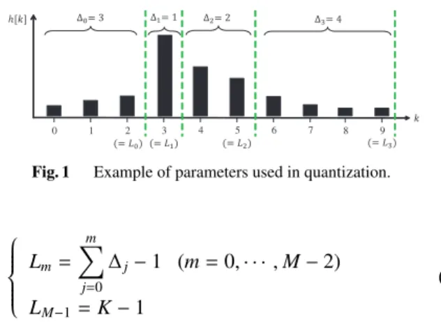
Fig. 1 Example of parameters used in quantization.













 Lm=

m

X

j=0

∆j−1 (m=0,· · ·,M−2) LM−1=K−1

(1)

Henceforth, them-th interval [Lm−(∆m−1),Lm] of the his- togram is called them-th bin. Since each bin has at least one element,Lm(0 ≤m≤M−2) is restricted to the following range:

m≤Lm≤K−(M−m) (2) Figure 1 illustrates the above-mentioned parameters for a histogram with ten elements (K = 10) quantized into four bins (M = 4). This figure shows that the bins contain 3(= ∆0) elements, 1(= ∆1) element, 2(= ∆2) elements, and 4(= ∆3) elements of the input histogram, and the upper boundaries of the bins areL0= ∆0−1=2,L1= ∆0+∆1−1= 3,L2 = ∆0+∆1+∆2−1=5, andL3= ∆0+∆1+∆2+∆3−1=9.

Quantizer design is based on minimizing the quantiza- tion error created by approximating all values in the m-th bin [L_m−(∆m−1),L_m] of the histogram with representative value ˆc(∆m,Lm). To assess the quantization error of them-th bin, we use the summation of square errore(∆m,L_m) defined as follows:

e(∆m,Lm)=

L_m

X

k=L_m−∆m+1

{k−c(ˆ∆m,Lm)}²h[k] (3) where ˆc(∆m,Lm) is the integer value that is closest to the centroid of them-th bin. The centroid is defined as follows:

c(∆m,L_m)= PLm

k=Lm−(∆m−1)kh[k]

PL_m

k=L_m−(∆m−1)h[k] (4) Optimizing the quantizer means finding the parameters that minimize the following summation of quantization error

(∆^∗₀,· · ·,∆^∗_M−1)= arg min

∆0,···,∆M−1











M−1

X

m=0

e(∆m,Lm)











(5)

2.2 M-Level Quantizer Design Based on Dynamic Pro- graming

Given that the quantization errore(∆m,L_m) of them-th bin depends on the boundary, Lm, of the m-th bin and the length, ∆m, of the same bin, dynamic programming based approaches (DP quantization) have been used to solve the optimization problem represented by Eq. (5).

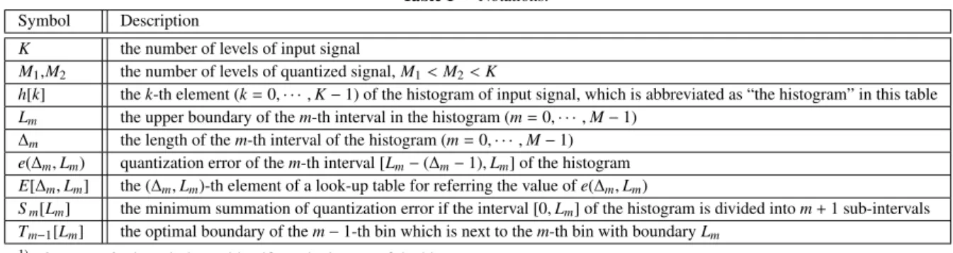
Table 1 Notations.

Symbol Description

K the number of levels of input signal

M₁,M2 the number of levels of quantized signal,M₁<M₂<K

h[k] thek-th element (k=0,· · ·,K−1) of the histogram of input signal, which is abbreviated as “the histogram” in this table L_m the upper boundary of them-th interval in the histogram (m=0,· · ·,M−1)

∆m the length of them-th interval of the histogram (m=0,· · ·,M−1) e(∆m,L_m) quantization error of them-th interval [Lm−(∆m−1),L_m] of the histogram E[∆m,L_m] the (∆m,L_m)-th element of a look-up table for referring the value ofe(∆m,L_m)

S_m[Lm] the minimum summation of quantization error if the interval [0,L_m] of the histogram is divided intom+1 sub-intervals Tm−1[Lm] the optimal boundary of them−1-th bin which is next to them-th bin with boundaryLm

1)Element indexis an index to identify each element of the histogram.

DP quantization focuses on the recurrence relation of quantization error. We define Sm[Lm] for each Lm (m = 0,· · ·,M−1) as the minimum summation of quantization errorPm

i=0e(∆i,Li) where interval [0,Lm] of histogramh[k]

(k=0,· · ·,K−1) is divided intom+1 bins. Sincee(∆m,Lm) depends on Lm and ∆m, Sm[Lm] can be expressed using Sm−1[Lm−∆m] given by the following recursive equation:

Sm[L_m]=min

∆m

{Sm−1[L_m−∆m]+e(∆m,Lm)} (6) wherem = 1,· · · ,M−1 andL_m = m,· · · ,K−(M−m).

Equation (6) says that computingSm[Lm] results in the se- lection of the best parameter among the values of ∆m = 1,· · ·,Lm−m +1. Solving Eq. (6) from m = 1 up to m=M−1 recursively, the minimization problem of Eq. (5) can be written as follows:

min∆M−1

{SM−2[LM−1−∆M−1]+e(∆M−1,LM−1)} (7)

2.3 Interpretation of Optimal Quantizer on Trellis Transi- tion Diagram

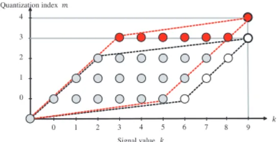
We use a trellis transition diagram to better explain the op- timization process of DP quantization. This interpretation will be useful in understanding the proposed algorithm de- scribed in Sect. 2.4. The trellis transition diagram of Fig. 2 illustrates the quantization result for the example shown in Fig. 1. The traversed path, indicated by the bold blue lines in Fig. 2, corresponds to the quantization result shown in Fig. 1. In Figd. 2, the vertical axis and the horizontal axis represent signal valuesk∈ {0,1,· · ·,9}to be quantized and quantization indicesm∈ {0,1,2,3}, respectively. The trellis transition diagram consists of nodes and paths. The node at (k,m) has a state wherein the interval [0,k] in the histogram is approximated withm+1 levels, and the upper bound of them+1-th bin is thek-th element of the histogram. The path from node (k−∆,m−1) to (k,m) has quantization er- ror of them-th bin corresponding to interval [k−∆ +1,k].

Thus, the design of the optimal quantizer that translates aK- level discrete signal into anM-level one can be represented as optimal path search from the node at (−1,−1) to that at (K−1,M−1) over the trellis transition diagram. Note that the node at (−1,−1) is a dummy node introduced as the start node and does not have the above-mentioned state.

Fig. 2 Traversed path corresponding to quantization shown in Fig. 1.

The transitions over the diagram need to satisfy the fol- lowing constraints:

(A) move one step in the upward direction per transition (B) move at least one step in the right direction per transi-

tion

Considering the above constraints, in the case of the quan- tization example (K = 10,M = 4) shown in Fig. 1, nodes that can be transited in the trellis transition diagram are re- stricted to those within the region delineated by broken-lines as shown in Fig. 2. This is generalized as follows: the nodes on the m-th row (m = 0,· · · ,M−2) exist in the range of k=m,· · ·,K−M+m.

2.4 Complexity Reduction for Designing Optimal Multi- Level Quantizers

We now turn to the design of the optimization of multiple quantizers that support multiple quantization levels. Our ex- ample is the optimization of an M1-level quantizer and an M2-level quantizer that both have as their inputs the same K-level signal (M1 < M2 < K). Note that although the following discussion deals with just two quantization lev- els, the same discussion applies to the general case of more than two levels without loss of generality. A straightforward approach to the design is to apply DP quantization to each quantization level independently. Hereinafter, this approach is referred to as simultaneous DP quantization. Simulta- neous DP quantization focuses on complexity reduction for a specific level of quantization. However, it does not ad- dress redundant computations between quantizers with dif- ferent quantization levels. To further reduce the complexity of multi-level quantizers, we focus on eliminating the redun-

Fig. 3 Trellis transition diagram for the example ofM=4 andM=5.

dant computations permitted by simultaneous DP quantiza- tion.

We introduce the basic concept of our proposal using the example shown in Fig. 3. In detail, we discuss a multi- level quantizer that quantizes a 10-level signal (K =10) to a 4-level signal (M₁ = 4) and a 5-level signal (M₂ = 5).

Figure 3 illustrates two trellis transition diagrams: one for 4-level quantization and one for 5-level. For the case of M1=4, traversed nodes are restricted to the white and gray nodes within the parallelogram area bounded by the black broken-lines. For the case ofM2 =5, traversed nodes are restricted to the red and gray nodes within the parallelogram area surrounded by the red broken-lines. The accumulated cost incurred by the gray nodes is the same for bothM1=4 andM2 =5. When we try to find the optimal quantizer for M2 = 5 after obtaining the optimal one for M1 = 4, it is not necessary to recompute the gray nodes for the case of M2 = 5. This is because those gray nodes are identical to those determined for M₁ = 4. For the case of M₂ = 5, it is sufficient to compute just the red nodes. This suppresses duplicate computation, which reduces complexity while re- taining solution optimality.

Generalizing the above example, let us consider the hi- erarchical optimization of anM1-level quantizer and anM2- level quantizer whose inputs are the same K-level signal.

The hierarchical optimization is designed assuming anM1- level quantizer that satisfies

(∆⁽¹⁾₀ ^∗,· · ·,∆⁽¹⁾_M1^∗₋₁)=arg min

∆0,···,∆M1−1











M₁−1

X

m=0

e(∆m,Lm)











(8) which is followed by anM2-level quantizer that satisfies

(∆⁽²⁾₀ ^∗,· · ·,∆⁽²⁾_M2^∗₋₁)=arg min

∆0,···,∆M2−1











M₂−1

X

m=0

e(∆m,Lm)











(9) TheM1-level quantizer is generated by solving Eq. (8) with DP quantization. The M2-level quantizer is generated by solving Eq. (9) with our improved DP quantization proposal that eliminates wasteful re-computation by reusing some of the results of DP quantization for the M1-level quantizer.

Basically, theM₂-level quantizer incurs accumulated costs ofSm[k] (m=0,· · ·,M2−2,k=m,· · ·,K−M+m) based on Eq. (6) in ascending order ofm. However, it is different from the M1-level quantizer in that not allSm[k] are computed from scratch. SinceSm[k] in the range of 0 ≤m≤ M1−2

are the same as those for theM1-level quantizer, they can be obtained by simply reusing the values computed for theM1- level quantizer. What needs to be computed from scratch for theM2-level quantizer is limited toSm[k] in the range of M₁−1≤m≤M₂−1. The above approach is referred to as layered DP quantization.

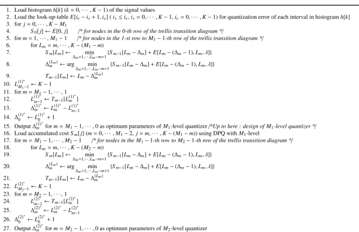
Figure 4 shows the pseudo-code of the multi-level quantizer stated above. Instruction 2 in Fig. 4 generates a look-up-table that stores the quantization error of every in- terval in the histogram. This look-up-table is shared be- tween M1-level quantizer and M2-level quantizer. Instruc- tions 3 to 15 correspond to the design of a M1-level quan- tizer using the DP quantization algorithm. In these pro- cesses, instructions 3 to 8 solve the minimization problem recursively based on Eq. (6), as described in Sect. 2.2. In- struction 9 stores the optimal boundary of them−1-th bin Lmin tableTm−1[Lm] for later reference. Instructions 10 to 14 obtain the optimal parameters (∆⁽¹⁾₀ ^∗,· · ·,∆⁽¹⁾_M−1^∗ ) from the following process, which is called the back-track process.

Since the possible value ofLM−1is limited toK−1, as the optimal value of LM−1, we have L⁽¹⁾_M−1^∗ = K−1. By using L⁽¹⁾_M−1^∗ =K−1 as a start point, and referring to tableTm[], we obtain L^∗_M−2 =TM−2[L^∗_M−1] ,· · ·,L^∗₀ =T₀[L^∗₁]. Using these valuesL⁽¹⁾_M−1^∗ ,· · ·,L⁽¹⁾₀ ^∗, we derive∆_M−1^(1)∗ =L⁽¹⁾_M−1^∗ −L⁽¹⁾_M−2^∗ , ,· · ·,

∆⁽¹⁾₁ ^∗=L⁽¹⁾₁ ^∗−L⁽¹⁾₀ ^∗,∆⁽¹⁾₀ ^∗ =L⁽¹⁾₀ ^∗+1 forM1-level quantizer.

Instructions 16 to 27 design the M2-level quantizer based on the algorithm provided in Sect. 2.4. Instruction 16 loads accumulated costs which are computed in generating theM₁-level quantizer. By reusing these accumulated costs, instructions 17 to 21 focus on m = M1−1,· · ·,M2 −1, i.e. the nodes in the restricted range among the M₁ −1- th row and the M2 −1-th row of the trellis transition dia- gram. Thus, we can eliminate the computations associated with m = 0,· · ·,M1 −2. Finally, the back-track process in instructions 21 to 27 generates the optimal parameters (∆⁽²⁾₀ ^∗,· · · ,∆⁽²⁾_M−1^∗ ) forM2-level quantizer.

3. Experiments

We performed the following experiments in order to inves- tigate the effectiveness of our quantization algorithm from the viewpoint of complexity reduction. As the input signal of each quantization algorithm, we used the sequences in ITE/ARIB Ultra-high definition/wide-color-gamut standard test sequences - Series A and Series B [23],[24]. The se- quences employ the progressive scan format with resolution of 3840×2160 pixels/frame in the RGB4:4:4 color format defined in ITU-R Recommendation BT.2020. These signals were sampled at 12 bit scale, so K = 4096. Green chan- nel signals of the head frame of each sequence were used in the following evaluation experiments. Given the existence of legacy displays, it is often necessary to convert high bit- depth signals into low bit-depth signals that have just ten or eight bits/channel. Accordingly, we setM = 1024,256 as the number of bins. These experiments were performed on a computer with an Intel core i7 CPU (2.8GHz) and 8GB of

1. Load histogramh[k] (k=0,· · ·,K−1) of the signal values

2. Load the look-up-tableE[ie−is+1,ie] (is≤ie,is=0,· · ·,K−1,ie=0,· · ·,K−1) for quantization error of each interval in histogramh[k]

3. forj=0,· · ·,K−M₁

4. S₀[j]←E[0,j] /* for nodes in the 0-th row of the trellis transition diagram */

5. form=1,· · ·,M1−1 /* for nodes in the 1-st row to M1−1-th row of the trellis transition diagram */ 6. forL_m=m,· · ·,K−(M1−m)

7. S_m[Lm]← min

∆m=1,···,L_m−m+1{S_m−1[Lm−∆m]+E[Lm−(∆m−1),L_m, λ]}

8. ∆^(Lm^m)←arg min

∆m=1,···,L_m−m+1{S_m−1[Lm−∆m]+E[Lm−(∆m−1),L_m, λ]}

9. T_m−1[Lm]←L_m−∆^(Lm^m)

10. L⁽¹⁾_M^∗

1−1←K−1 11. form=M1−1,· · ·, 1 12. L^(1)∗

m−1←T_m−1[L⁽¹⁾m^∗] 13. ∆⁽¹⁾m^∗←L⁽¹⁾_m^∗−L^(1)∗

m−1

14. ∆⁽¹⁾0 ^∗←L⁽¹⁾₀ ^∗+1

15. Output∆⁽¹⁾m^∗form=M₁−1,· · ·,0 as optimum parameters ofM₁-level quantizer/*Up to here : design of M₁-level quantizer */ 16. Load accumulated costS_m[j] (m=0,· · ·,M1−2,j=m,· · ·,K−(M1−m)) using DPQ withM1-level

17. form=M₁−1,· · ·,M₂−1 /* for nodes in the M₁−1-th row to M2−1-th row of the trellis transition diagram */ 18. forL_m=m,· · ·,K−(M2−m)

19. S_m[Lm]← min

∆m=1,···,Lm−m+1{S_m−1[Lm−∆m]+E[Lm−(∆m−1),L_m, λ]}

20. ∆^(Lm^m)←arg min

∆m=1,···,L_m−m+1{S_m−1[Lm−∆m]+E[Lm−(∆m−1),L_m, λ]}

21. T_m−1[Lm]←L_m−∆^(Lm^m)

22. L^(2)∗

M2−1←K−1 23. form=M₂−1,· · ·, 1 24. L^(2)∗

m−1←T_m−1[L⁽²⁾_m^∗] 25. ∆⁽²⁾m^∗←L⁽²⁾_m^∗−L⁽²⁾_m−1^∗ 26. ∆⁽²⁾₀ ^∗←L^(2)∗

0 +1

27. Output∆⁽²⁾m^∗form=M₂−1,· · ·,0 as optimum parameters ofM₂-level quantizer

Fig. 4 Optimal design of multi-level quantizer withM₁/M₂-level using multi-layered DP quantiza- tion.

memory.

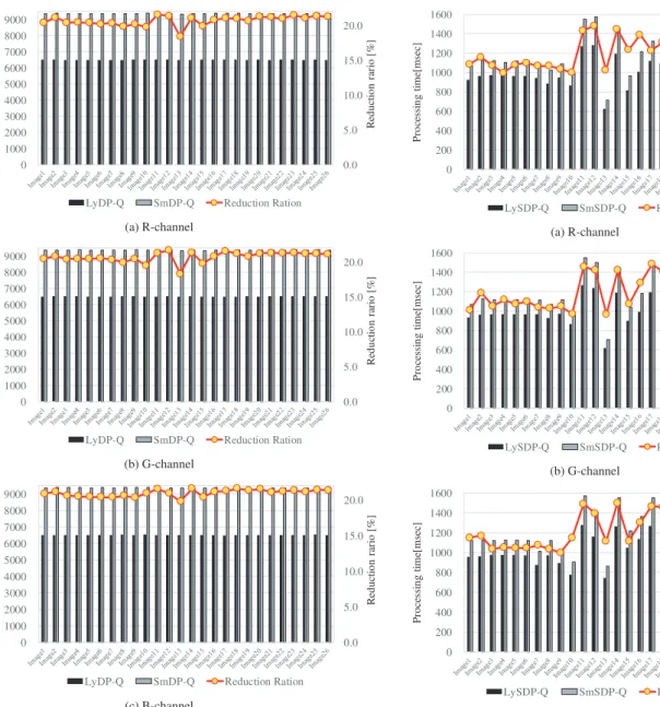
In order to evaluate the complexity reduction achieved by layered DP quantization (abbreviated as LyDP-Q), we compared LyDP-Q with simultaneous DP-quantization (ab- breviated as SmDP-Q) in terms of running time. As we described in 2.4, SmDP-Q designs two optimal quantizers for M = 1024 and M = 256 by applying DP quantization to each quantization level M = 1024,256 independently.

By contrast, LyDP-Q supports the elimination of duplicate computations between different quantization levels. For this comparison, we calculated the following metric:

complexity reduction ratio=

running time of SmDP-Q−running time of LyDP-Q

running time of SmDP-Q (10)

The results are shown as bar graphs in Fig. 5, where gray bars and black bars represent the running time of SmDP- Q and LyDP-Q, respectively. We confirmed that LyDP-Q yielded a 20.8% (on average) complexity reduction over SmDP-Q. The proposed algorithm leads to computation effi- ciency while keeping the optimality of multi-level quantiza- tion in terms of minimizing the total amount of quantization error.

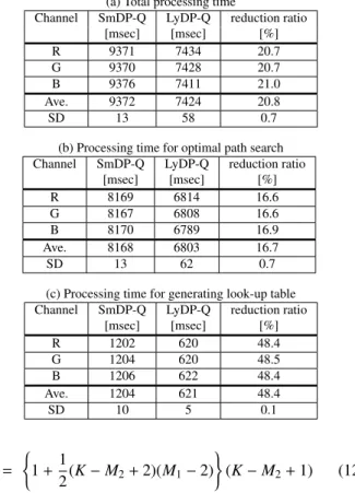
Furthermore, our layered approach can be incorporated into sparse DP quantization (SDP-Q)[17]in the same way as DP quantization. Figure 6 shows the running time of our layered approach built on SDP-Q (abbreviated as LySDP-Q)

and the simultaneous approach built on SDP-Q (abbreviated as SmSDP-Q). We confirmed that LySDP-Q had less com- plexity, 16.1% on average, than SmSDP-Q. SDP-Q pays at- tention to the amplitude sparseness of signal values for com- plexity reduction, whereas our layered approach focuses on inter-level redundancy. Therefore, as the above results show, our layered approach well complements the conventional complexity reduction scheme for DP quantization.

The proposed method with its layered strategy achieved its complexity reduction by eliminating the follow- ing computations:

(C1) duplicated processes to search for optimal paths for M2-level quantization

(C2) duplicated generation of a look-up table E[] for M2- level quantization

Further details on the complexity reduction are to be found in Table 2. Table 2(a) shows average processing time of SmDP-Q and LyDP-Q for all images. The figures in col- umn “reduction ratio” in Table 2(a) were computed by ap- plying the same concept as Eq. (10) to the candidate paths of SmDP-Q and LyDP-Q. As a breakdown of the process- ing time of both algorithms, Tables 2(b) and (c) give the processing time for searching optimal path and that for gen- erating look-up tables, respectively. As a countermeasure to the above-mentioned “C1”, LyDP-Q reused a part of the computations performed for M1-level quantization for opti-

Fig. 5 Running time of LyDP-Q and SmDP-Q (“reduction ratio” is de- fined in (10)).

mizingM₂-level quantization. As a result, LyDP-Q reduced the processing time of this process by 16.7% over SmDP- Q, as shown in Table 2(b). This contributed to reduce the total processing time by 14.6%. As a countermeasure to the above-mentioned “C2”, LyDP-Q shared the look-up ta- ble of the M1-level quantization with theM2-level quanti- zation instead of generating look-up tables for each quan- tization. This is because the look-up table of the M1-level quantization includes that of theM2-level quantization. As a result, LyDP-Q reduced the processing time of this pro- cess by 48.4% over SmDP-Q, as shown in Table 2(c). This contributed to reduce the total processing time by 6.2%.

Next, we analyze the complexity of the above- mentioned “C1” and “C2” for the approach based on DP quantization which is abbreviated as DP-Q. The complex- ity of “C1” is related to the number of feasible paths within

Fig. 6 Running time of LySDP-Q and SmSDP-Q (“reduction ratio” is defined by Eq. (10)).

the search range that is shared among both quantizations.

In the following, feasible paths within the search range are abbreviated as candidate paths, and candidate paths that are shared between both quantizations are abbreviated as shared candidate paths. According to[17], the number of candidate paths for DP-Q that quantizes aK-level signal into aM-level signal is derived as follows:

Ωpath(M,K)

= 1

2M³−2K+5

2 M²+K²+7K+4

2 M−K²−K (11) The number of shared candidate paths for DP-Qs that output M1-level/M2-level signals fromK-level signal is derived as follows:

Ωshared-path(M1,M2,K)

Table 2 Average processing time of SmDP-Q and LyDP-Q for all im- ages (cells in the “reduction ratio” columns present the values yielded by Eq. (10), and cells in the SD rows present standard deviations of all chan- nels).

(a) Total processing time

Channel SmDP-Q LyDP-Q reduction ratio

[msec] [msec] [%]

R 9371 7434 20.7

G 9370 7428 20.7

B 9376 7411 21.0

Ave. 9372 7424 20.8

SD 13 58 0.7

(b) Processing time for optimal path search Channel SmDP-Q LyDP-Q reduction ratio

[msec] [msec] [%]

R 8169 6814 16.6

G 8167 6808 16.6

B 8170 6789 16.9

Ave. 8168 6803 16.7

SD 13 62 0.7

(c) Processing time for generating look-up table Channel SmDP-Q LyDP-Q reduction ratio

[msec] [msec] [%]

R 1202 620 48.4

G 1204 620 48.5

B 1206 622 48.4

Ave. 1204 621 48.4

SD 10 5 0.1

= (

1+1

2(K−M2+2)(M1−2) )

(K−M2+1) (12) The derivation of the above equation can be found in Appendix.

Based on these analysis models, we found that com- plexity reduction obtained by eliminating “C1” is evalu- ated asΩshared-path(M1,M2,K); it reflects the complexity- related computations reused in searching for optimal paths of M2-level quantization. Furthermore, the reduction ratio which is the above complexity reduction over the complex- ity relevant to this process in SmDP-Q is evaluated as fol- lows:

CRpash(M₁,M₂,K)= Ωshared-path(M₁,M₂,K) Ωpath(M1,K)+ Ωpath(M2,K)

(13) For the case ofK = 4096,M2 =1024 and M1 =256, the reduction ratio is 17.9%, which is close to the simulation results shown in the rightmost column in the “Ave.” row of Table 2(b). Additionally, the standard deviations of the processing time were small as shown in the “SD” row in the table.

The complexity of “C2” is related to the number of can- didate intervals in the input histogram, because the quanti- zation error of each candidate interval needs to be computed and stored inE[]. According to[17], the number of candi- date intervals for DP-Q that quantizes aK-level signal into aM-level signal is derived as follows:

Ωinterval(M,K)=(−M²+M+K²+K)/2 (14) Based on this analysis model, we found that complex- ity reduction obtained by eliminating “C2” is evaluated as Ωinterval(M₂,K); the complexity for generating the look- up table ofM2-level quantization. Furthermore, the reduc- tion ratio which is the above complexity reduction over the complexity relevant to this process in SmDP-Q is evaluated as follows:

CRinterval(M1,M2,K)

= Ωinterval(M₂,K)

Ωinterval(M1,K)+ Ωinterval(M2,K) (15) For the case ofK =4096,M2 =1024 andM1 =256, the reduction ratio is 48.5%, which agrees well with the simu- lation results shown in the rightmost column in the “Ave.”

row of Table 2(c). Additionally, the standard deviations of the processing time were small as shown in the “SD” row in the table.

The above analysis for two-layer quantization can be generalized to two or more layers. LetLandMldenote the number of layers and the quantization level of thel-th layer (l = 1,· · ·,L), respectively. Note that M1 < M2 < · · · <

ML. In the case of anL-layer quantization, letting M^(L) = (M1,· · ·,ML), the reduction ratio of Eq. (13) is generalized to

CRpath(M^(L),K)= PL

l⁰=2Ωshared-path(Ml⁰−1,Ml⁰,K) PL

l=1Ωpath(Ml,K) The above is derived in the followings. The num- ber of candidate paths of LyDP-Q is Ωpath(M1,K) + PL

l⁰=2

nΩpath(M_l⁰,K)−Ωshared-path(M_l⁰−1,M_l⁰,K)o

. On

the other hand, the number of candidate paths of SmDP-Q is PL

l=1Ωpath(Ml,K). So, the reduction of the former with re- spect to the latter isPL

l⁰=2Ωshared-path(Ml⁰−1,Ml⁰,K), and we obtain the above reduction ratio. Similarly, the reduction ratio of Eq. (15) is generalized to

CRinterval(M^(L),K)= PL

l⁰=2Ωinterval(Ml⁰,K) PL

l=1Ωinterval(M_l,K)

This is because the candidate intervals ofM1contain all can- didate intervals ofM2,· · ·,ML.

Table 3 provides comparisons between SmSDP-Q and LySDP-Q. Table 3(a) shows average processing time of SmSDP-Q and LySDP-Q for all images. The figures in the column “reduction ratio” in Table 3(a) were computed by applying the same concept as Eq. (10) to the candidate paths of SmSDP-Q and LySDP-Q. Table 3(b) and (c) give the processing time for searching for the optimal paths and that for generating look-up tables, respectively. As a result, LySDP-Q reduced the time taken by this process by 14.0%

over SmSDP-Q, as shown in Table 3(b). This contributed to reducing the total processing time by 12.6%. LyDP-Q reduced the processing time of this process by 33.4% over

Table 3 Average processing time of SmSDP-Q and LySDP-Q for all images (cells in the “reduction ratio” column present values given by Eq. (10)).

(a) Total processing time

Channel SmSDP-Q LySDP-Q reduction ratio

[msec] [msec] [%]

R 1252 1054 15.9

G 1263 1061 16.0

B 1311 1097 16.3

Ave. 1276 1071 16.1

(b) Processing time for optimal path search Channel SmSDP-Q LySDP-Q reduction ratio

[msec] [msec] [%]

R 1122 966 13.9

G 1131 973 14.0

B 1173 1006 14.3

Ave. 1142 982 14.0

(c) Processing time for generating look-up table Channel SmSDP-Q LySDP-Q reduction ratio

[msec] [msec] [%]

R 130 87 32.9

G 132 88 33.1

B 138 91 34.0

Ave. 133 89 33.4

SmDP-Q, as shown in Table 3(c). This contributed to reduc- ing the total processing time by 3.5%.

It was observed that the reduction ratio of LySDP-Q was less than that of LyDP-Q from the perspectives of total processing time, processing time of optimal path search, and processing time to generate look-up table.

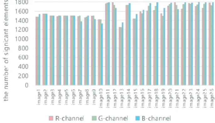
We consider the cause of this observation by analyz- ing the complexity of “C1” and “C2” for approaches based on SDP-Q. Since SDP-Q skips insignificant elements in the histogram of the input signal, the number of insignificant elements impacts the complexity of approaches based on SDP-Q, such as SmSDP-Q and LySDP-Q. The number of significant elements varies depending on channels of im- ages used in our experiments as shown in Fig. 7. This is why the processing times of SmSDP-Q and LySDP-Q de- pend on images in Fig. 6. In the following, let ˜K be the number of the significant elements. Based on the analy- sis models of Eqs. (11) and (12), the complexity reduction gained by eliminating “C1” is approximately evaluated as Ωshared-path(M1,M2,K). The reduction ratio which is the˜ above complexity reduction over the complexity relevant to this process in SmSDP-Q is approximately evaluated as fol- lows:

Ωshared-path(M1,M2,K)˜

Ωpath(M1,K)˜ + Ωpath(M2,K)˜ (16) The number of significant elements depends on the in- put signal. In the following, let us consider the complexity of SmSDP-Q and LySDP-Q using the average number of significant elements over all input signals (26 kinds of im- ages) used in the experiments. The average number of the significant elements was 1597. In the case of ˜K = 1597,

Fig. 7 The number of insignificant elements in each channel.

M2 =1024 andM1 =256, the above analytical evaluation says that the reduction ratio would be 10.5%. This value is less than the reduction ratio of K = 4096, M2 = 1024 andM1 =256, which was 48.5% as stated previously. This shows that the reduction ratio tends to decrease as the num- ber of significant elements decreases. This trend closely re- sembles the experimental results. There was, however, some gap between the analytical evaluation and the simulation re- sults shown in the rightmost column in Table 3(c). This is because Eqs. (12) and (11) are analytical models for DP-Q based approaches and can not exactly represent the number of candidate paths for SDP-Q. Specifically, the analytical models do not consider the complexity reduction achieved by restricting the search range, see Sect. 5.2 in[17].

Based on this analysis model of Eq. (14), the complex- ity reduction achieved by eliminating “C2” is approximately Ωinterval(M2,K). The reduction ratio which is the above˜ complexity reduction over the complexity relevant to this process in SmDP-Q is evaluated as follows:

Ωinterval(M2,K)˜

Ωinterval(M₁,K)˜ + Ωinterval(M₂,K)˜ (17) In the case of ˜K = 1597, M₂ = 1024 andM₁ = 256, the above analytical evaluation says that the reduction ratio is 37.7%, which is close to simulation results shown in the rightmost column of Table 3(c).

4. Conclusion

This paper extended DP quantization so as to significantly reduce the complexity of multi-level quantization. The al- gorithm proposed herein eliminates the redundant compu- tations between different quantization levels without los- ing the optimality of multi-level quantization. Experiments showed that the proposed algorithm attained 20.8% and 16.1% lower complexity (on average) than simultaneous quantization built on DP quantization and sparse DP quan- tization, respectively.

References

[1] R.M. Gray and D.L. Neuhoff, “Quantization,” IEEE Trans. Inf. The- ory, vol.44, no.6, pp.2325–2383, Oct. 1998.

[2] E. Reinhard, G. Ward, S. Pattanaik, P. Debevec, W. Heidrich, and K. Myszkowski, High Dynamic Range Imaging: Acquisition, Dis- play, and Image-Based Lighting, 2nd ed., Morgan Kaufmann Pub- lisher, 2010.

[3] E. Franc¸ois, D. Rusanovskyy, P. Yin, P. Topiwala, G. Sullivan, and M. Naccari, “Signalling, backward compatibility and display adap- tation for HDR/WCG video coding, draft 1,” ISO/IEC JTC1/SC29/ WG11/N16508, Oct. 2016.

[4] A. Artusi, T. Richter, T. Ebrahimi, and R.K. Mantiuk, “High dy- namic range imaging technology [lecture notes],” IEEE Signal Pro- cess. Mag., vol.34, no.5, pp.165–172, Sept. 2017.

[5] J. Boyce, Y. Ye, J. Chen, and A. Ramasubramonian, “Overview of SHVC: Scalable extensions of the high efficiency video coding standard,” IEEE Trans. Circuits Syst. Video Technol., vol.26, no.1, pp.20–34, 2016.

[6] ISO/IEC, Information technology: Scalable compression and coding of continuous-tone still images – Part 1: Scalable compression and coding of continuous-tone still images, ISO/IEC 18477-1, 2015.

[7] ISO/IEC, Information technology: Scalable compression and coding of continuous-tone still images – Part 8: Lossless and nearlossless coding, ISO/IEC 18477-8, 2016.

[8] E. Franc¸ois, C. Fogg, Y. He, X. Li, A. Luthra, and A. Segall, “High dynamic range and wide color gamut video coding in HEVC: Sta- tus and potential future enhancements,” IEEE Trans. Circuits Syst.

Video Technol, vol.26, no.1, pp.63–75, 2016.

[9] ISO/IEC, Information technology: Scalable compression and coding of continuous-tone still images – Part 2: Coding of high dynamic range images, ISO/IEC 18477-2, 2016.

[10] ISO/IEC PDTR 23008-14: Information technology — High effi- ciency coding and media delivery in heterogeneous environments — Part 14: Conversion and Coding Practices for HDR/WCG Y’CbCr 4:2:0 Video with PQ Transfer Characteristics, 2016.

[11] A.O. Zaid and A. Houimli, “HDR image compression with op- timized JPEG coding,” European Signal Processing Conference, pp.1539–1543, Aug. 2017.

[12] S.P. Lloyd, “Least squares quantization in PCM,” IEEE Trans. Inf.

Theory, vol.IT-28, pp.129–136, March 1982.

[13] J. Max, “Quantizing for minimum distortion,” IRE Trans. Inf. The- ory, vol.IT-7, pp.7–12, March 1960.

[14] J.D. Bruce, Optimum quantizer, Ph.D. thesis, M.I.T., May 1964.

[15] D. Sharma, “Design of absolutely optimal quantizers for a wide class of distortion measures,” IEEE Trans. Inf. Theory, vol.24, no.6, pp.693–702, Nov. 1978.

[16] X. Wu, “Optimal quantization by matrix searching,” J. Algorithms, vol.12, no.4, pp.663–673, Dec. 1991.

[17] Y. Bandoh, S. Takamura, and A. Shimizu, “Sparse DP quantization algorithm,” IEICE Trans. Fundamentals, vol.E102-A, no.3, pp.553–

565, March 2019.

[18] ITU-T and ISO/IEC JTC 1, High efficiency video coding, ITU-T Rec.H.265 and ISO/IEC 23008-2(HEVC), version 6, June 2019.

[19] ITU-T and ISO/IEC JTC 1, Advanced Video Coding for Generic Audio-Visual Services, ITU-T Rec.H.264 and ISO/IEC 14496-10 (AVC), version 13, June 2019.

[20] Y. Bandoh, S. Takamura, and A. Shimizu, “Complexity reduction of multi-level DP quantization through inter-level redundancy elimina- tion,” Proc. IEEE Int. Conf. Image Process., WP.PF.1, 2019.

[21] D. Muresan and M. Effros, “Quantization as histogram segmenta- tion: Optimal scalar quantizer design in network systems,” IEEE Trans. Inf. Theory, vol.54, no.1, pp.344–366, 2008.

[22] A.K. Khandani, “A hierarchical dynamic programming approach to fixed-rate, entropy-coded quantization,” IEEE Trans. Inf. Theory, vol.42, no.4, pp.1298–1303, 1996.

[23] http://www.ite.or.jp/content/test-materials/uhdtv a/ [24] http://www.ite.or.jp/content/test-materials/uhdtv b/

Appendix: Derivation of Eq. (12)

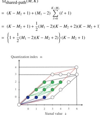
Let us consider the candidate paths shared among two DP- Qs that output M₁-level/M₂-level signal from the sameK- level signal. We evaluate the shared candidate paths in two cases:

(i) nodes in a range withm=0

(ii) nodes in a range withm=1,· · ·,M₁−2

Figure A·1 illustrates the case ofK =7,M2=5 andM1 = 4. The green nodes and the blue nodes represent the nodes in class (i) and class (ii), respectively. First, let us consider class (i). In this class, there areK−M2+1 kinds of nodes, and every node has a single path. Accordingly, we find that there areK−M₂+1 kinds of paths. Figure A·1 shows the paths in this class as the green line segments. Second, let us consider class (ii). In this class, a node (m+`,m) has`+1 kinds of paths. In a group of nodes located at (m+`,m) where` =0,1,· · ·,K−M2,m =1,· · ·,M1−2, there are the following number of paths:

M1−2

X

m=1 K−M2

X

`=0

(`+1)=(M1−2)

K−M2

X

`=0

(`+1)

Figure A·1 shows the paths in this class as the blue line segments. From the above results, we obtain the following:

Ωshared-path(M,K)

= (K−M2+1)+(M1−2)

K−M2

X

`=0

(`+1)

= (K−M2+1)+1

2(M1−2)(K−M2+2)(K−M2+1)

= (

1+1

2(M1−2)(K−M2+2) )

(K−M2+1)

Fig. A·1 Shared nodes in the case ofK=7,M2=5 andM1=4.

Yukihiro Bandoh received the B.E., M.E., and Ph.D. degrees from Kyushu University, Japan, in 1996, 1998 and 2002, respectively. He granted JSPS Research Fellowship for Young Scientists from 2000 to 2002. In 2002, he joined Nippon Telegraph and Telephone (NTT) Corpo- ration, where he has been engaged in research on efficient video coding for high realistic com- munication. He is currently a Distinguished En- gineer at NTT Media intelligence Laboratories.

Dr. Bandoh is a senior member of IEEE, IEICE, and IPSJ.

Seishi Takamura received the B.E., M.E.

and Ph.D. degrees from the University of To- kyo in 1991, 1993 and 1996, respectively. In 1996 he joined Nippon Telegraph and Telephone (NTT) Corporation, where he has been engaged in research on efficient video coding and ultra- high quality video coding. He has fulfilled var- ious duties in the research and academic com- munity in current and prior roles including As- sociate Editor of IEEE Transactions on Circuits and Systems for Video Technology, Executive Committee Member of IEEE Tokyo Section, Japan Council and Region 10, and Vice President-Industrial Relations and Development of APSIPA. He has also served as Chair of ISO/IEC JTC 1/SC 29 Japan National Body, Japan Head of Delegation of ISO/IEC JTC 1/SC 29, and as an International Steering Committee Member of the Picture Coding Symposium. From 2005 to 2006, he was a Visiting Scientist at Stanford University, California, USA. He is currently a Senior Distinguished Engineer at NTT Media Intel- ligence Laboratories. Dr. Takamura is a Fellow of IEEE, a senior member of IEICE and IPSJ, and a member of MENSA, APSIPA, SID and ITE.

Hideaki Kimata received the B.E. and M.E.

degrees in applied physics, and the Ph.D. degree in electrical engineering respectively from Na- goya University, Nagoya, Japan, in 1993, 1995, and 2006. He joined Nippon Telegraph and Telephone Corporation (NTT) in 1995, and has been involved in the research and development of video coding, realistic communication, com- puter vision, and video recognition based on ma- chine learning (deep learning). He is currently a Senior Research Engineer and also the Supervi- sor at NTT Media Intelligence Laboratories. He is a Chair of Technical Committee on Image Engineering of the Institute of Electronics, Informa- tion and Communication Engineers of Japan.