Shallow-groundwater-temperature-fluctuations near the water table in the paddy fields showed by the fourier series-香川大学学術情報リポジトリ

(1)

Vol 20, No 1 (1968)

SHALLOW-GROUNDWATER-TEMPERATURE-FLUCTUATIONS

NEAR THE WATER TABLE

IN

THE PADDY FIELDS SHOWED BY THE FOURIER SERIES

Kiyoshi FUKUBA Katsuhiko

Izursu

and

Tadao

MAEKAWA

1. Introduction

In order to show mathematically the periodic functions in a problem of physics or engineering, the most familliar periodic functions of sin x, cos x, tan x, etc. are generally used

The monthly average shallow-groundwater-temperature-fluctuations near the water table during a year (shown by crosses in Figs. 2, 3 and 4) also have periodic fluctuations. Therefore we applied the FOURIER series to a periodic function in order to show the fluctuation of the shallow groundwater temperature (G. T.) and obtained a result. The paper presented here shows the result and is the 13th report on "shallow groundwater in the downstream basin of the Aya River".

2. Theory

In order to find an equation whose value of G.T. varies but little from the observed ones (shown by crosses in Figs 2, 3 and 4), we used harmonic analysis ( 2 )

.

At first, we confined the problem to estimating: 1) the temperature of shallow groundwater near the water table, and 2) the average temperature for a given area.

We made the interval [O,2n] correspond to the length of a year (12 months) and divided it into 12 equal parts (12 months) by the points

or in degrees

The values of the observed G,T. or 0 at these points (or every month) are known to be

where Oo = 0 in January 0 = 0 in February 0 2 =0 in March

...

Bl 1 = B in December

1

(2)

86 Tech. Bull. Fac. Agr. Kagawa Univ.,

Thus we have, for the theoretical values of G.T., by using the FOURIER series ( 3 )

,

= O , I , 2 ,

...

11.

= I , 2,

...

6.

where

-

denotes approximate equality.

In this case, it is easy to see that all the factors multiplying the ordinates in Eqs. (6) and (7) reduce to

0, f I , f sin 30' = f 0.5, f sin 60' = f 0.866

and it is easily verified that

For convenience of calculation in obtaining the approximate values of Ot, we rewrote Eq.(5) into Eq. (20).

ao n 2n

O t = -talcos - 2x4-a2 cos -2n+ . . . . , . o . . , , , ' .

6n

I2 12

+

a6 cos - 2n

n 2 I2

n 2n

+bl sin

-

2n +b2 sin

-

2n+

..---.--.---

+b5 sin

-

5n 2n.

...

(3)

Vol. 20, No. 1 (1968) 87

3. Data

The observed values of

G.T.

(or 0) used to calculate the values of a012 and the FOURIER coefficients (Eqs.(7) and (8) are shown in Figs. 2, 3 and 4 (crosses)). The observed values of

G.T.

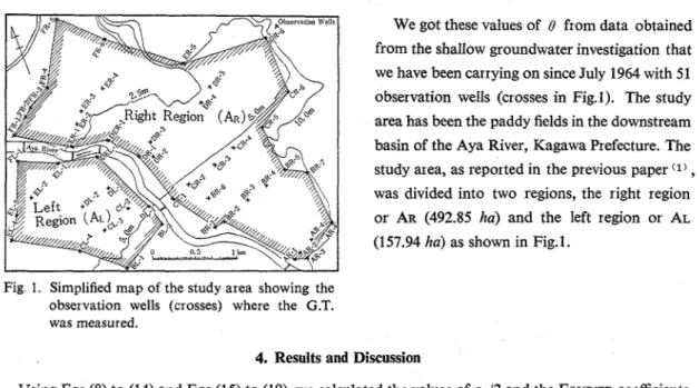
(or 8) used to estimate the theoretical values of G.T. (0t) by using Eq.(20) are also shown in Figs. 2 , 3 and 4 (crosses). From the curves shown in these figures, we see that the values of 8 fluctuate periodically.

We got these values of 0 from data obtained from the shallow groundwater investigation that we have been carrying on since July 1964 with 51 observation wells (crosses in Fig.1). The study area has been the paddy fields in the downstream basin of the Aya River, Kagawa P~efecture. The study area, as reported in the previous paper (1)

,

was divided into two regions, the right region or AR (492.85 ha) and the left region or AL (1 57.94 ha) as shown in Fig. I .

Fig 1 Simplified map of the study axea showing the observation wells (crosses) where the G.T.

was measured.

4. Results and Discussion

Using Eqs.(8) to (14) and Eqs.(l5) to (19), we calculated the values of a012 and the FOURIER coefficients (al, a2, a s , ad, a5

,

a s , bl

,

bz

,

b3

,

b4 and b 5 ) as listed in Table 1.

Table 1 Values of the FOURIER coefficients as calculated by Eqs. (8) to (19). We used these values to obtain the theoretical values of G.T. shown in Figs. 2, 3 and 4.

(4)

88 Tech Bull Fac Agr. Kagawa Univ.

Using Eq.(20) with the values listed in Table 1, we calculated the theoretical values of G.T. (Bt) for AR for every month during 1965. The results are shown by the open circles in Fig.2 (1965, AR).

In like manner (by using Eq.(20)), we obtained the values of Bt for AL and Aw during the same year. The values of Ot for 1966 and 1967 were also calculated as shown in Figs. 3 and 4 respectively.

Fig. 2.

Theoretical values (open circles) and the observed values (crosses) of G T. for AR, AL and Aw during 1965.

T (Month)

I

25

: 1 9 6 6 : Fig. 3.

- A1

:

Theoretical values (open

20 - ₁_{circles) and the observed}

values (crosses) of G.T

.O 1 5 - for AR, AL and Aw during

< 1966 a . 10 25

-

10 I I I I I I I I I I J F M A M J J A S O N D T (Month)

(5)

Vol. 20, No. 1 (1968)

J F h l A M J J A S O N D

T (Month)

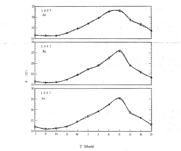
Fig. 4.. Theoretical values (open circles) and the observed values (crosses) of G..T. for AR, AL and Aw during 1967.

Looking at the curves shown in Figs. 2, 3 and 4, we see that the theoretical values of G.T. or O t (open circles) are close to the observed ones (crosses) for every region for every month throughout the entire three years.

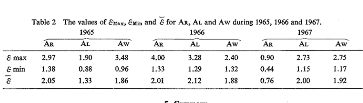
To see how much the theoretical values of G. T. ( O t ) deviate from the observed ones ( 0 ) in every month, we used Eq.(21) and estimated the values of the deviation (E). Their major values are listed in Table 2.

From the values listed in Table 2, we see that the maximum values of & or are below 4.00

%;

the minimum values of & or E ~ i n are below 1.18

%;

and the mean values of & or

E

are below 2.12% for

(6)

Tech, Bull. Fac. Agr

.

Kagawa Univ..

Table 2 The values of EM%=, i in and for AR, AL and Aw during 1965,1966 and 1967.

1965

_-

1966 1967 0h AL Aw

.

, AR AL Aw

.

.AR

AL Aw

.

E max 2.97 1.90 3.48 4.00 3.28 2.40 0.90 2.73 2.75 Emin 1.38 0.88 0.96 1.33 1.29 1.32 0.44 1.15 1.17 - E 2.05 1.33 1.86 2.01 2.12 1.88 0.76 2.00 1.92 5. Summary

Using the FOURIER series, we obtained a theoretical equation, Eq.(20), that showed the shallow groundwater temperature (monthly average) fluctuation near the water table for a year.

The values calculated by Eq.(20) were close t o the observed ones as shown in Figs. 2, 3 and 4. 6. Acknowledgements

The writers wish t o thank t o the Emeritus Professor Dr. Hitoshi FUKUDA and Professor Dr. Hiroyuki OGATA, both of Tokyo University, for their encouragement.

References

(1) FUKUDA, K., NAGANO, T., MAEKAWA, T.: Tech. matics, 208-213, John Wiley & Sons, Inc., New Y o ~ k Bull. Fac. Agr. Kagawa Univ., 18, No. 2 186-207, (1961)-

(1967). (3) To~srov, G.P.: FOURIER series, 150-152, Pren-

(2) REDDICK, H.W., MILLER, F.H.: Advanced Mathe- tice-Hall, Inc., Englewood Cliffs, New Jersey (1965).

FOURIER

& B T S B

Lf:7J(ffl&%O~T$EM;fE@EB&T7J(BOgB

z?

r.

a

7kEa&tCCb;V6&T7kfiWZDER&7;7kaCt,

l+Rd%DRdB%Rt%'-, c?r DZ@S~ID@&% FOURIER BRLV:ZtB%, Eq. (201, CCk o T 6 % L k

5

t%&t:

et

6

( R B ~

&-F/~P (OCI

t

$6

t,

2n

er=*fal cos n 2 n . t a 2 cos

-

2n+ 6n

12 12 f a 6 cos - 2n

n 2 12

2n

+bl sin 2ni-bz sin

-

2n+ 5n

12 12 f b a sin - 12 2n (20)

n=O, 1, 2,

,

11 ( n = O i i l A , n = l l t 2 A ,

,

n=116;f;12AbZ%GT6)

2 Z CC, %it Eqo (8) t C k 9 T , 37: FOURIER &V& a ~ , a2,

,

ae B k U bl, 62,

,

bsbi,

+

hQh

Eqs. (9)-(19) CZk

-T$XGhQ

SNIE

(0, OC) (1965-1967~) ~G.ZCZR,A L

et

s

21 3 L.~CF,+SB, ~ B Z D 3 ~ ~ ~ P L V Z ~ B L T ,

et

i t

e

t

k

<

-

Z? L (Figs. 2, 3 2 1 7 3 4 1, -? DB%tt, Eq. (21) b2 k T%$?T8

2,

4 % U T ,

TQIibT

2.12%HTT &of:.

3BCCRtV: ( & 6 A D ) Ri%!J4LCt, @E&!I@ ( B l l l R @ l l l T R % D 7 k ~ & t , 650 79ha) Vt3D51i%!JA

tZ#'F,

Fig. 1) T , (+DA 42) Lt: m m (mS51) DBi%4!ibD%@jF% (&@&bfiD$%) !ET&

Q