Lyαスペクトルで探る遠方星形成銀河のアウトフロー

(1)

Outflows in Distant Star Forming Galaxies

Probed by Lyman Alpha Spectra

(

Ly

αスペクトルで探る遠方星形成銀河のアウトフロー

)

Takuya Hashimoto

橋本拓也

　　　　　東京大学大学院理学系研究科天文学専攻

平成２６年１２月　博士（理学）申請

(2)

Outflows in Distant Star Forming Galaxies

Probed by Lyman Alpha Spectra

(

Ly

αスペクトルで探る遠方星形成銀河のアウトフロー

)

35-127074

Takuya Hashimoto

橋本拓也

Department of Astronomy, Graduate School of Science

The University of Tokyo

(3)

(4)

(5)

Abstract

In galaxy formation and evolution, gas exchanges between galaxies and the ambient intergalactic medium (IGM), i.e., outflows and inflows, are thought to play important roles. Outflows have been ubiquitously found in nearby and high redshift (high-z) galaxies. However, at high-z, outflow studies are limited in luminous massive galaxies such as Lyman Break Galaxies (LBGs). While some authors have argued the importance of outflows from low mass galaxies in chemical enrichment (e.g., Larson, 1974), the presence and properties of outflows in them are not well examined due to their faintness.

Recently, Nakajima et al. (2012) have constructed the largest Lyman Alpha Emitter (LAE) photometry sample at z ∼ 2.2 containing as many as ∼ 4000 LAEs. LAEs are selected by virtue of their strong Lyα emission. Previous studies have shown that LAEs are less massive than other galaxy populations at the same redshift. Several spectroscopic follow-up observations have been performed to detect rest-frame UV and optical lines which are essential for understanding outflows. Thanks to these observations, now it is practical to inspect the presence of outflows in LAEs. In this thesis, we first examine the presence of outflows in 12 LAEs at z ∼ 2.2 based on high spectral resolution Lyα data taken by Magellan/MagE (R ∼ 4000) and Keck/LRIS (R ∼ 1100), and nebular emission lines by Magellan/MMIRS, Keck/NIRSPEC, and Subaru/FMOS. Specifically, a Lyα line of four objects have been obtained by MagE, that of six objects by LRIS, and that of two objects by the both spectrographs. We have detected both Lyα and nebular emission lines in all the 12 objects. In a stacked spectrum of the four MagE spectra, we have also detected several low ionization state (LIS) metal absorption lines in LAEs for the first time (Hashimoto et al. 2013). LIS absorption lines are additionally detected in three individual spectra of LRIS object (Shibuya et al. 2014a). In order to probe outflows in LAEs, after determining the systemic velocity from nebular emission lines, we examine the velocity properties of Lyα and LIS absorption lines. We have confirmed that all the 12 objects have a main Lyα peak redward of the systemic, and 5 out of the 12objects additionally

(6)

have a weak Lyα emission blueward of the systemic, so called “blue bump”. We find that most of the Lyα profiles are asymmetry with a red tail and a blue sharp cut oﬀ, and the main red peak is redshifted with respect to the systemic velocity by ∆vLyα,r ≃ 200 km

s−1_{. Finally, we have measured the blueshift of LIS absorption lines with respect to the}

systemic redshift, to find that they are blue shifted by |∆vabs| ≃ 100 − 200 km s−1. These

three results are all consistent with a scenario that LAEs have outflows. Thus, we have confirmed the presence of outflows in LAEs with a large sample and several techniques.

The finding that LAEs have outflows is also important to understand Lyα escape mech-anisms in LAEs. Many theoretical works have investigated how galaxy properties aﬀect the Lyα escape and emergent Lyα profile. Using a Monte Carlo technique, the Lyα ra-diation transfer has been in general computed through idealized spherically symmetric shells of homogeneous and isothermal neutral hydrogen gas. The ultimate goal of these studies is to understand the physical nature of galaxies using the Lyα line. Several works have compared observed Lyα lines with those predicted by models both in LBGs (e.g., Verhamme et al. 2008; Kulas et al. 2012) and LAEs (Chonis et al. 2013). Verhamme et al. (2008) have shown that their expanding shell model can well reproduce observed Lyα profiles. On the other hand, Kulas et al. (2012) and Chonis et al. (2013) have argued that such models can not reproduce observed Lyα lines well, especially the position and flux of a blue bump. There are some problems to be solved in these studies. First, Ver-hamme et al. (2008) have determined the best fit model parameters by eye, not by the statistics. This prevents one from estimating errors of the best-fit parameters, as well as examining degeneracies among the parameters. Second, Kulas et al. (2012) have fitted a stacked spectrum of 12 LBGs. As recently pointed out by several authors, stacking analysis generates an imaginary spectrum rather than a typical spectrum of the 12 LBGs. It is possible that the discrepancies are caused by the stacking analysis. Finally, while Chonis et al. (2013) have fitted three individual Lyα spectra, those spectra have similar Lyα profiles and Lyα luminosities. This also prevents them from a definitive conclusion of the origin of the discrepancies. In addition to these problems, Kulas et al. (2012) and Chonis et al. (2013) have not compared the best fit parameters with observables.

In this thesis, we have applied the Lyα radiative transfer code constructed by Verhamme et al. (2006) and Schaerer et al. (2011) to our data on the individual basis. Unlike the sample in Chonis et al. (2013), our 12 objects have a wide variety of Lyα profiles and Lyα luminosities. We also determine the best-fit parameters and their associated errors from the χ2 _{statistics. In addition, since various observables of our objects have been}

(7)

the problems in previous studies. We also try to understand our finding in Hashimoto et al. (2013) that LAEs have smaller ∆vLyα,r than those in LBGs. From this, we infer

the key properties on Lyα escape mechanisms. We have found that all the Lyα profiles in our objects are well reproduced. For the objects without blue bump, model parameters are broadly consistent with the observables. However, for objects with the blue bump, we find that an intrinsic FWHM of Lyα, FWHMint(Lyα), is significantly larger than that of

nebular lines. We infer that the parameter FWHMint(Lyα) is the key to well reproduce

observed profiles. We propose that if we introduce an additional source of Lyα emission such as gravitational cooling, the large FWHMint(Lyα) and the existence of the blue bump

can be simultaneously explained. We have then examined four possibilities of the origin of small ∆vLyα,rin LAEs: a large galactic outflow velocity, the presence of a peculiar ISM

with a unity covering fraction, CF = 1, a patchy ISM with a neutral gas covering fraction below unity, CF < 1, and the low neutral hydrogen column density (NHi)of the gas. We

find that the small ∆vLyα,rcan be quantitatively well explained by the low NHi scenario.

Their typical NHi is as low as log(NHi) ∼ 1019 cm−2, which is more than one order of

magnitude lower than that in LBGs. Such a low column density could be consistent with the recent findings of LAEs having high ionization parameter (Nakajima & Ouchi 2014) or low Hi gas mass (Pardy et al. 2014). Thus, we show quantitatively that NHi is the key

for the Lyα escape in LAEs for the first time.

We finally discuss two implications for reionization studies. First, in estimating the neutral fraction of the IGM from Lyα emissivity, ∆vLyα is assumed to be 400 km s−1. If

LAEs at z > 6 have similarly small ∆vLyα,rvalues as derived in this study, the amount of

Lyα photons scattered by the IGM, as used to constrain the epoch of reionization, may be in need of revision. Second, from our finding that high EW(Lyα) objects tend to have small ∆vLyα,rand the finding in Verhamme et al. (2014) that objects with ionizing photon

leaking should have small ∆vLyα,r, we propose that targeting high EW(Lyα) objects would

(8)

(9)

List of Figures

2.1 Nebular Emission Line Spectra Taken by MMIRS and NIRSPEC . . . . 16

2.2 Nebular Emission Line Spectra Taken by FMOS . . . 17

2.3 Lyα Line Spectra Taken by MagE . . . 19

2.4 Lyα Line Spectra Taken by LRIS . . . 20

3.1 Comparison between Lyα and Nebular Emission Lines in the Velocity Space: MagE Data . . . 26

3.2 Comparison between Lyα and Nebular Emission Lines in the Velocity Space: LRIS Data . . . 27

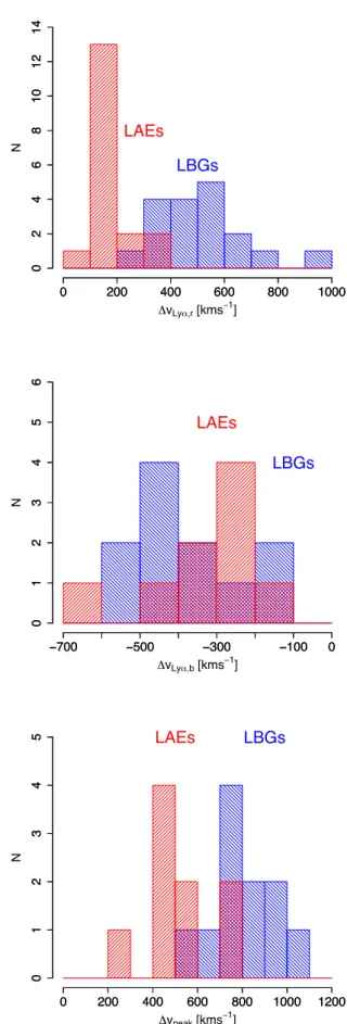
3.3 Histograms of Three Lyα Velocity Oﬀsets, ∆vLyα,r, ∆vLyα,b, and ∆vpeak for LAEs and LBGs . . . 30

3.4 Rest-frame EW(Lyα) as a function of ∆vLyα,r . . . 31

3.5 Composite FUV Spectrum of the Four LAEs . . . 34

3.6 Two Component [Oiii] λ5007 Profiles . . . 35

3.7 Results of SED Fitting . . . 40

4.1 Determination of the Best Fit and its Associated Errors using χ2_values ₄₇ 4.2 The Best-fit Reproduced Profiles . . . 49

4.3 Examples of 2D χ2 _{contours to examined degeneracy among parameters:} Vexp and log(NHI) . . . 52

4.4 Examples of 2D χ2 _{contours to examined degeneracy among parameters:} τa and b . . . 53

4.5 Examples of 2D χ2 _{contours to examined degeneracy among parameters:} EWint(Lyα) and FWHMint(Lyα) . . . 54

4.6 Comparison between Observables and Model Parameters: Galactic Out-flow Velocity . . . 56 4.7 Comparison between Observables and Model Parameters: Dust Extinction 57

(14)

4.8 Comparison between Observables and Model Parameters: Full Width at Half Maximum of Lines . . . 58 4.9 The Best-fit Reproduced Profiles Fixing their Intrinsic Lyα FWHM as

FWHM(neb) . . . 59 4.10 Comparison between Observables and Model Parameters: Equivalent Width 60

5.1 ∆vLyα,r as a function of Covering Fraction of the ISM . . . 69

5.2 ∆vLyαas a function of the neutral hydrogen column density of the uniform

(15)

List of Tables

2.1 Summary of our observations . . . 22

3.1 Summary of the spectroscopic properties of the sample . . . 24

3.2 Summary of the Two Component Fit for [Oiii] λ5007 Lines . . . 36

3.3 Broadband Photometry of Our Sample . . . 38

3.4 Results of SED fitting . . . 39

3.5 Summary of Morphological Properties . . . 42

4.1 Model Parameter Values . . . 45

4.2 Summary of the Lyα Fitting for the Sample . . . 50

(16)

(17)

Chapter 1

Introduction

1.1 Galaxies

Galaxies are self-gravitating systems consisting of stars, interstellar medium (ISM), dust, and dark matter. Galaxies show variety of appearance from ordered disk-like elliptical shapes to irregular shapes. Since they are a basic component of the Universe, it is im-portant to understand how they evolved with time. How can we study past galaxies ? Because the speed of light is limited, one can study them by observing distant galax-ies. Selecting distant galaxies from a literally “astronomical” number of objects in the sky is the first step to study them. The most direct and secure way to determine the distance to objects is spectroscopy. One can determine it by measuring how much spec-tral lines are shifted into longer wavelengths with respect to their rest-frame wavelengths (redshift; z). However, the number of objects which can be simultaneously observed by spectroscopy is limited. In addition, due to the sensitivity limit, it is quite diﬃcult to perform spectroscopy for faint objects. Instead, using the characteristic galaxy Spectral Energy Distributions (SEDs), two photometric techniques are commonly used to search for high redshift (high-z) galaxies as described below.

1.2 High-Redshift Galaxies

1.2.1 Lyman Break Galaxies

Young massive O- and B-type stars in star forming galaxies eﬃciently emit ionizing pho-tons (λ ≤ 912 ˚A). Those photons are absorbed by neutral hydrogen atoms in the inter stellar medium (ISM) and used for their ionization. In addition to that, photons with

(18)

λ≤ 1215.67 ˚A are resonantly scattered by neutral hydrogen in the inter galactic medium (IGM) along the line of sight. The break in SEDs at λ ≤ 1215.67 ˚A made by these two eﬀects is called Lyman Break. Thus, using the color excess between two broad-bands, one at the wavelength λ! 1215.67 ˚A and the other at λ" 1215.67 ˚A, one can eﬃciently select star forming galaxies. Star forming galaxies selected in this technique are called Lyman Break Galaxies (LBGs). Large surveys have found thousands of LBGs from z ∼ 2 up to z! 10 (e.g., Ellis et al. 2013) and have revealed that they are moderately massive galaxies (1010 _{- 10}11 _M

⊙ Shapley et al. 2004; Erb et al. 2006b). A weak point of this method is

that FUV continuum has to be detected, which introduce a selection bias toward UV bright objects.

1.2.2 Lyman Alpha Emitters

Another technique to search for high-z galaxies uses the Hi Lyα line (λrest = 1215.67˚A).

Lyα is the most prominent UV emission line, and is emitted when an electron falls from quantum level n = 2 to n = 1. It is produced by several astronomical phenomena; recombination radiation following photoionization by young massive O- and B type stars in Hii regions (e.g., Partridge & Peebles 1967) and by fluorescence in intergalactic medium (IGM) (e.g., Cantalupo et al. 2005; Kollmeier et al. 2010), collisional excitation radiation following gravitational cooling (e.g., Faucher-Gigu`ere et al. 2010; Rosdahl & Blaizot 2012). The Lyα technique uses the color excess of Lyα against FUV continuum, where Lyα emission is observed by a narrow band filter and FUV continuum by a broadband filter. Objects selected by this method, with large Lyα equivalent width of EW(Lyα)_{! 20 − 30} ˚

A, are called Lyα Emitters (LAEs). The merit of this technique is that one can eﬃciently search for galaxies very faint in continuum emission (i.e., low mass objects). LAEs are now commonly seen in both the local and high-z universes (local: Deharveng et al. 2008; Cowie et al. 2011, high-z: Hu & McMahon 1996; Rhoads & Malhotra 2001; Ouchi et al. 2008, 2010). Previous studies based on SED have revealed that typical LAEs are low-mass galaxies with a small dust content (" 109_M

⊙ e.g., Nilsson et al. 2007; Gawiser et al. 2007;

Guaita et al. 2011; Nakajima et al. 2012), although there are some evolved LAEs with moderate mass and dust (Ono et al. 2010a; Hagen et al. 2014). Morphological studies have shown that LAEs are typically compact (e.g., Bond et al. 2009, 2010) and their typical size does not evolve with redshift (Malhotra et al. 2012). Thus, LAEs are among the building block candidates in the Λ Cold Dark Matter (CDM) model, where smaller

(19)

contrast to their importance in galaxy evolution and formation, their properties are not fully understood due to their faintness.

1.3 Previous Studies Related to LAEs

In §1.2.2, we have summarized what are LAEs and their basic properties revealed by their SEDs and morphologies. In this section, first, we briefly summarize the previous studies utilizing LAEs which examine the high-z large scale structure (§1.3.1) and the epoch of cosmic reionization (§1.3.2). Then, we summarize recent studies which examine properties of LAEs (§1.3.3).

1.3.1 Clustering Analysis of LAEs

Each galaxy is enveloped by a dark matter halo, a self-gravitating system composed of dark matter. Therefore, studying dark matter halo masses and their redshift evolution leads to understanding the history of stellar mass assembly. While it is diﬃcult to directly investigate them, theoretical studies have shown that a massive dark matter halo has stronger clustering strength (e.g., Sheth & Tormen 1999, Mo&White 02). The clustering strength of dark matter halos can be probed by those of galaxies. In fact, utilizing the extremely large field view of e.g., Subaru/Suprime-Cam, previous studies have discovered numerous LAEs and analyzed their clustering strength (e.g., Ouchi et al. 2008; Guaita et al. 2010). These studies have revealed that LAEs reside in dark matter halos which are among the lowest mass halos at a given redshift.

1.3.2 LAEs as a Probe of Cosmic Reionization

380,000 years after the Big Bang (z ∼ 1100), ionized hydrogen experienced recombination due to the expansion and cooling of the Universe. Since there are no stars nor galaxies, this is called the “dark age” of the Universe. On the other hand, it is known that the Universe is fully ionized, indicating that the Universe is re-ionized by UV ionizing photons emitted by stars and galaxies at some epoch. This is called “cosmic reionization”. However, how and when reionization has happened are not fully understood. The nature of ionizing sources is also an open question.

(20)

Fan et al. (2006) have examined absorption in high-z QSOs continua at wavelengths shorter than 1215.67 ˚A. This technique utilizes the resonant nature of Lyα: QSO contin-uum emission is seen redshifted as 1215.67˚A and is absorbed by the neutral hydrogen in the foreground IGM. Thus, this probes the neutral fraction of the IGM, xHI, between the

QSOs and us. They have shown that reionization has completed as late as z ∼ 6.

LAEs are also used as a probe of reionization because the Lyα line is sensitive to xHI. We

introduce two methods related to LAEs commonly used in reionization studies. First one is to examine the evolution of the Lyα luminosity function. At the epoch of reionization (EoR), the observed number density of LAEs should be decreased because Lyα photons are scattered by neutral hydrogen atoms in the IGM. Indeed, Kashikawa et al. (2006); Ouchi et al. (2010); Kashikawa et al. (2011) have demonstrated that the Lyα luminosity function rapidly decreases from z = 5.7 to z = 6.6. Taking into account the fact that UV luminosity function remains unchanged during this period (e.g., Kashikawa et al. 2011), these results indicate that reionization has been completed at z _{! 6. Second one is to} investigate the evolution of the fraction of galaxies with Lyα emission among LBGs, Lyα fraction. Stark et al. (2010, 2011) have shown that lower UV luminosity LBGs have larger Lyα fractions, and that the fraction increases from z ∼ 4 to z ∼ 6. However, later studies (e.g., Ono et al. 2012; Schenker et al. 2012, 2014) have demonstrated that the fraction decrease from z ∼ 6 to z ∼ 8. This is also interpreted as a result of a rapid increase in xHI, from being fully ionized at z ∼ 6 to a volume-averaged neutral fraction as high as

∼ 60% at z ∼ 8 (Jensen et al. 2013; Stark et al. 2014).

1.3.3 Recent Findings of LAEs

Until recently, near-infrared spectroscopy for LAEs is quite diﬃcult due to their faintness. It is not until 2011 that nebular emission lines have been successfully detected in LAEs (McLinden et al. 2011; Finkelstein et al. 2011). Since then, thanks to the recent advent of high sensitivity near-infrared spectroscopy instruments, and to the establishment of LAE catalogues for the nebular emission line spectroscopy, the number of LAEs whose nebular emission lines have been detected is rapidly increasing. Finkelstein et al. (2011) have successfully derived the gas phase metallicity in two z ∼ 2 LAEs for the first time using the 1σ upper limit on the [Nii] flux with the N2 index (e.g., Pettini & Pagel 2004). They have claimed that at least one LAE does not obey to the well-established mass-metalliciy relation (e.g., Tremonti et al. 2004; Erb et al. 2006a) in the sense that it has much lower

(21)

Nakajima et al. (2013) have remarkably succeeded in deriving both gas phase metallicity and gas ionization parameter using the diagram of the R23 index versus the [Oiii]/[{sc Oii] flux ratio (Pagel et al. 1979; Kewley & Dopita 2002). They have shown that LAEs have lower gas phase metallicity and higher gas ionization parameter than those of LBGs. These findings are further confirmed by Nakajima & Ouchi (2014) with a large sample containing both local and high-z galaxies.

Several studies have investigated the position of LAEs in the diagram of star formation rate against stellar mass. It is known that normal star-forming galaxies make a main sequence whereas starburst galaxies such as ULIRGS and/or submm galaxies lie above the main sequence (e.g., Daddi et al. 2007). Therefore, the diagram is useful to understand the mode of star formation. Hagen et al. (2014) have examined stellar populations of bright LAEs discovered by HETDEX pilot survey. Interestingly, they have found that those LAEs are burst-like galaxies (see also Chonis et al. 2013; Rhoads et al. 2014; Vargas et al. 2014). Recently, Kusakabe et al. (2014) have investigated rest-frame IR luminosity to examine dust properties of LAEs utilizing Spitzer/MIPS 24 µm and Herschel/PACS data. They have found that rather than Calzetti dust extinction law (Calzetti et al. 2000) which is commonly adopted, the Small Magellanic Cloud attenuation curve (Pettini et al. 1998) is more appropriate for the averaged LAEs. After carefully correcting SFR for dust extinction, they have claimed that at least the averaged LAEs are consistent with the main sequence.

1.4 Open Questions concerning LAEs

We describe two open questions concerning LAEs: the presence of outflows and the Lyα photon escape mechanism.

1.4.1 The Presence of Outflows

Gas exchanges between galaxies and the ambient intergalactic medium (IGM), i.e., out-flows and inout-flows, are thought to play important roles in galaxy evolution. Outout-flows are driven by supernovae (SNe), stellar winds from massive stars, and AGN activity (Heckman et al., 1990; Murray et al., 2005; Choi & Nagamine, 2011). Galaxies which lost cold gas via outflows may experience a reduction or even termination of subsequent star formation. In contrast, cold gas supplied by inflows may increase the star formation, especially when

(22)

they come in the form of dense, filamentary gas streams (‘cold accretion’; e.g. Dekel et al. 2009). Gas exchanges will also aﬀect the chemical evolution of galaxies and the IGM, and thus have played important roles in establishing the mass-metalliciy relation across cosmic time (e.g., Larson 1974; Tremonti et al. 2004; Erb et al. 2006a; Yabe et al. 2015). Outflows have been found in nearby starburst galaxies (Heckman et al., 1990), nearby ULIRGs (Martin, 2005), LBGs at z ∼ 2 − 3 (Pettini et al., 2002; Shapley et al., 2003), and BX/BM galaxies at z ∼ 2 (Steidel et al., 2010). These studies have made use of the fact that FUV low-ionization interstellar (LIS) absorption lines, which are generated when continuum photons encounter the outflowing gas, are blue-shifted with respect to the systemic redshift measured by nebular emission lines such as Hα originated from Hii regions in the galaxy.

Examining the incidence of outflows in LAEs is of interest, because LAEs are generally low mass galaxies and thus have shallow gravitational potentials. Some authors have argued the importance of outflows from less massive galaxies in chemical enrichment (e.g., Larson, 1974). However, FUV continua of LAEs are too faint for LIS absorption lines to be reliably measured with current facilities.

Lyα is also used to probe the gas kinematics. The Lyα line is known to have complex profiles caused by its resonant nature. Many theoretical and observational studies have shown that outflowing gas leads to a redshifted Lyα line with respect to the systemic redshift (e.g., Verhamme et al., 2006; Steidel et al., 2010), giving a positive Lyα oﬀset velocity, ∆vLyα,r. This also leads to an asymmetric Lyα profile with a red tail and a blue

sharp cut oﬀ. In the case of an outflow, back-scattered (i.e., redshifted) Lyα photons have more chance of escape because they drop out of resonance with the foreground gas. However, it is very diﬃcult to obtain high-resolution nebular emission spectra for LAEs because they are faint compared to strong sky emission.

Prior to Hashimoto et al. (2013), only four LAEs have both high-resolution Lyα and nebular line spectra: two from McLinden et al. (2011) and two from Finkelstein et al. (2011). Objects in McLinden et al. (2011) have ∆vLyα,r = 125 ± 17.3 and 342 ± 18.3

km s−1_{, respectively, and objects in Finkelstein et al. (2011) have ∆v}_Lyα,r _{= 288 ±}

37 (photometric) ± 42 (systematic) and 189 ± 35 ± 18 km s−1_{, respectively. The fact}

that all four have ∆vLyα,r > 0 suggests that outflows are common in LAEs. However,

due to the small sample sizes obtained so far, there has not been a statistical discussion of the gas motions of LAEs. The presence of outflows in LAEs should be examined with a larger sample.

(23)

1.4.2 The Lyα Escape Mechanism

Another important question in LAEs is their Lyα escape mechanism. Due to the resonant nature of Lyα photons, Lyα photons would be easily absorbed by dust grains after their long light paths. However, LAEs have strong Lyα emission, suggesting that they have low dust extinction and/or some mechanisms that make light paths of Lyα photons short. Taking into account the fact that a large fraction (75%) of young galaxies have strong Lyα emission (Cowie et al. 2011), studying the Lyα escape mechanism is important for understanding the physical nature of galaxies at the early stage of galaxy evolution.

Some observational studies at the local universe have proposed that outflows facilitate the escape of Lyα photons from galaxies (e.g., Kunth et al., 1998) as they reduce the number of resonant scattering. Likewise, others (e.g., Kornei et al. 2010; Atek et al. 2014) have shown that dust content correlates with Ly escape fraction. While these eﬀect would certainly at work, there has been no decisive conclusion.

On the other hand, using a Monte Carlo technique, the Lyα radiation transfer (RT) has been in general computed through idealized spherically symmetric shells of homogeneous and isothermal neutral hydrogen gas. These theoretical studies have investigated how galaxy properties aﬀect the Lyα escape and emergent Lyα profiles. These studies have shown that Lyα RT is a complicated process altered by galactic outflows/inflows (e.g., Verhamme et al. 2006; Dijkstra & Loeb 2009), the neutral hydrogen column density and dust content of the ISM (e.g.,Zheng & Miralda-Escud´e 2002; Verhamme et al. 2006), and the inclination of the galaxy disk (e.g., Verhamme et al. 2012; Zheng & Wallace 2014), as well as by the properties of the IGM surrounding the galaxy (e.g., Kollmeier et al. 2010; Laursen et al. 2013). One of the goals in these theoretical studies is to aid understanding the galaxy properties from the observed Lyα line, and to identify the key factors for the Lyα escape.

To understand Lyα RT and escape by a close comparison of observed and modeled Lyα lines, it is important to obtain spectral lines other than the Lyα line. The line centroid and the velocity dispersion of nebular emission lines (e.g., Hα and [Oiii]) oﬀer information on the galaxy’s systemic redshift and an internal motion of Hii regions, respectively. On the other hand, as described above, a blue-shift of LIS metal absorption lines with respect to the systemic redshift reveals the galactic outflow velocity, and the width of the LIS lines can be interpreted as the thermal velocity of the outflowing gas. These lines would

(24)

disentangle the complicated Lyα RT and help to understand the Lyα escape. However, as described in §1.4.1, it has been diﬃcult to obtain LIS metal absorption lines nor nebular emission lines in LAEs.

Recent successful detections of both Lyα and nebular emission lines have opened up studies which compare observed and modeled Lyα lines in the context of a spherical outflowing gas shell not only in LBGs (e.g., Verhamme et al. 2008; Kulas et al. 2012) but also in LAEs (Chonis et al. 2013). On one hand, utilizing the shell model constructed by Zheng & Miralda-Escud´e (2002) and Kollmeier et al. (2010), Kulas et al. (2012) and Chonis et al. (2013) have shown that the expanding shell model can not well reproduce observed Lyα profiles, especially a secondary emission blue-ward of the systemic velocity. On the other hand, based on the expanding shell model constructed in Verhamme et al. (2006), Verhamme et al. (2008) have shown that the expanding shell model can well reproduce observed profiles as well as other observed properties such as the dust content. There are, however, some problems to be solved in these studies. First, the best fit parameters in Verhamme et al. (2008) have been determined by eye, not by the statistics. This prevent us from determining the best fit parameters and its associated errors, as well as the degeneracy among the parameters. Second, Kulas et al. (2012) have compared a stacked spectrum of 12 LBGs with modeled Lyα lines. As recently pointed out by several authors (e.g., Vargas et al. 2014), stacking analysis provides a poor representation of individual objects. This would cause a discrepancy between observed and modeled Lyα lines. On the other hand, Chonis et al. (2013) have compared observed and modeled Lyα lines on the individual basis for three objects. As described in Chonis et al. (2013), these three objects have very similar Lyα profiles and Lyα luminosities. Thus, a larger sample with various Lyα profiles and physical properties (e.g., stellar mass, Lyα luminosity) is needed, in order to understand how well the expanding shell model can reproduce observed Lyα profiles and observables. This question is quite important because many observational studies make use of the expanding shell model to interpret observed Lyα profiles. Since Kulas et al. 2012; Chonis et al. 2013 could not fitted their Lyα profiles, there has been no discussion related to Lyα escape mechanism in these studies. Thus, first we need to quantitatively examine the validity of the expanding shell, then investigate the Lyα escape mechanisms.

As we show in §3, we examine the Lyα and absorption velocity properties and compare them with those of LBGs. Interestingly, LAEs and LBGs have similar velocity properties except for ∆vLyα,r. LAEs have ≃ 200 km s−1 which is significantly smaller than those in

(25)

Hashimoto et al. (2013) have shown that ∆vLyα,r anti-correlates with EW(Lyα), which

is confirmed with larger samples in Shibuya et al. (2014a) and Erb et al. (2014). Thus, understanding the origin of the small ∆vLyα,r through the detailed Lyα modeling should

shed light on the Lyα RT and escape in LAEs.

1.5 Open Questions Concerning Cosmic Reionization

Understanding high-z LAEs properties such as the Lyα escape mechanism is also impor-tant for reionization studies.

As described in §1.3.2, some studies utilizing LAEs have suggested that the neutral fraction of IGM, xHI, has rapidly increased from being fully ionized at z ∼ 6 to a

volume-averaged neutral fraction as high as ∼ 60% at z ∼ 8 (Jensen et al. 2013; Stark et al. 2014). However, some theoretical studies point out that it is unphysical that the neutral fraction of the IGM has changed in such a short period. Indeed, aforementioned studies have put some assumptions when deriving xHI. In particular, related to this thesis, these studies

have assumed that Lyα lines are redshifted with respect to the systemic by ∆vLyα,r∼ 400

km s−1_{when they enter the IGM out of the galaxy (see also Santos 2004). If Lyα photons}

with a large ∆vLyα,r enter the IGM, they would suﬀer less scattering since they are out of

resonance from the neutral hydrogen in the IGM. Thus, without the exact value of ∆vLyα,r,

one cannot precisely derive the neutral fraction of the IGM. However, it is quite diﬃcult to obtain ∆vLyα,r at such a high-z before the advent of James Webb Space Telescope (but

see Stark et al. 2014). Therefore, it is quite important to systematically study ∆vLyα,r at

lower redshift such as z ∼ 2.

Recently, several studies have investigated potential ionizing sources of reionization by searching for galaxies with ionizing photon leaking (Lyman Continuum; LyC). LyC emission is detected in LAEs and LBGs both spectroscopically (Shapley et al. 2006) and photometrically (e.g., Iwata et al. 2009; Nestor et al. 2013). In particular, Iwata et al. (2009) have demonstrated that the ionizing photon escape fraction is higher in LAEs than that in LBGs. Taking into account the fact that LAEs are the dominant population at high-z, they would have significantly contributed to reionization. This picture is further supported by the finding of Nakajima et al. (2013) and Nakajima & Ouchi (2014). They have shown that LAEs have the highest ionization parameter (i.e., the number of ionizing photons per a neutral atom) in a large sample of local and z ∼ 2−3

(26)

galaxies. Verhamme et al. (2014) and Behrens et al. (2014) have examined Lyα profiles for two possible LyC leaking scenarios: (1) galaxies with density bounded Hii regions where ionizing photons completely ionize the ISM, (2) galaxies with a neutral ISM with holes. They have demonstrated that the Lyα oﬀset with respect to the systemic redshift, ∆vLyα,r,

should be quite small in these cases. Since LAEs have small ∆vLyα,r, it is interesting to

understand their Lyα profiles closely to examine a possible connection between LAEs and galaxies with high LyC escape fractions.

1.6 Goals of This Thesis

As described, LAEs are low mass galaxies and are important not only in understanding galaxy evolution and formation, but also in cosmic reionization studies. However, due to their faintness, properties such as the presence of outflows and the Lyα escape mechanism have not been fully understood. This also prevents us from putting a strong constraint on EoR.

In order to address these questions, in this thesis, we use the largest (N ≃ 4000 objects) z∼ 2.2 LAE samples in the COSMOS, the Chandra Deep Field South (CDFS), and the Subaru/XMM-Newton Deep Survey (SXDS) (Nakajima et al. 2012, 2013, and Nakajima et al. in prep.). These LAE samples are all based on Subaru/Suprime-Cam imaging observations with our custom made narrow band filter, NB387 (λc = 3870˚A and FWHM

= 94˚A). The redshift of z ≃ 2.2 is favored since we can simultaneously observe Lyα, LIS absorption lines (e.g., [Siii]), [Oi], and [Cii]), and optical nebular lines (e.g., [Oii], Hβ, [Oiii], and Hα) from the ground. Furthermore, we can compare the kinematics and Lyα radiative transfer of LAEs with those of brighter and more massive galaxies at similar redshifts, e.g., LBGs, obtained by previous studies.

We performed several follow-up spectroscopy observations for the samples. High spec-tral resolution Lyα lines are obtained by Magellan/MagE (R ∼ 4000) and Keck/LRIS (R ∼ 1100), and nebular emission lines by Magellan/MMIRS, Keck/NIRSPEC, and Sub-aru/FMOS. Specifically, Lyα spectra of four objects have been obtained by MagE, that of six objects by LRIS, and two objects by both spectrographs. As a result, we have successfully detected both Lyα and nebular emission lines for the 12 objects. LIS metal absorption lines are additionally detected in a stacked spectrum of the four MagE spectra and three LRIS individual spectra.

(27)

Lyα main peak with respect to the systemic redshift for the 12 objects. As described above, in the case of an outflow, the Lyα profile should be asymmetric with a positive

∆vLyα,r. In addition, for the objects with LIS absorption lines, we also measure their

blueshift with respect to the systemic redshift, ∆vabs. Since there are only four (no)

objects with measured ∆vLyα,r (∆vabs) (McLinden et al. 2011; Finkelstein et al. 2011)

prior to Hashimoto et al. (2013), the spectra of the 12 objects enable us to discuss the presence of outflows with the highest confidence.

After confirming the presence of outflows in LAEs, we apply the Monte Carlo based Lyα radiative transfer code constructed by Verhamme et al. (2006) and Schaerer et al. (2011) to our data. This enables us (1) to examine how well the shell model can reproduce observed Lyα profiles, and (2) to understand the Lyα RT and escape mechanism in LAEs. Concerning the first point, we compare observed and modeled Lyα profiles on an in-dividual basis. Unlike the sample in Chonis et al. (2013), our 12 objects have a wide variety of Lyα profiles and physical quantities such as stellar masses derived from SED fitting. In addition, we determine the best-fit parameter and its associated error from the χ2 _{statistics unlike Verhamme et al. (2008) who have determined the best-fit parameter}

by eye.

Concerning the second point, Hashimoto et al. (2013) have remarkably shown that the mean value of ∆vLyα,r is significantly smaller than those of LBGs (e.g., Steidel et al.

2010; Kulas et al. 2012) even at the same stellar mass, star formation rate, and velocity dispersion of nebular lines. In addition, as we show in §3, velocity properties of Lyα and absorption lines reveal that the only significant diﬀerence in the velocity properties between LAEs and LBGs is ∆vLyα,r. Understanding it would shed light on the Lyα escape

mechanism in LAEs. Theoretical studies propose four possibilities of the origin of small

∆vLyα,r in LAEs: a large galactic outflow velocity, the presence of a peculiar ISM with

a unity covering fraction, CF = 1, a patchy ISM with a neutral gas covering fraction below unity, CF < 1, and the low neutral hydrogen column density (NHI) of the gas. By

comparing with results of theoretical studies, we examine the origin of the small ∆vLyα,r

in LAEs. Erb et al. (2014) have recently successfully detected both Lyα and nebular emission lines for as many as 26 LAEs. They have also found that LAEs have small

∆vLyα,r and tried to interpret it. However, their Lyα profiles have much lower spectral

resolution compared with ours, which prevents them from a close comparison with RT models. Our high resolution Lyα spectra enable us to discuss the origin of it much more

(28)

quantitatively than Erb et al. (2014).

Finally, we discuss implications for reionization studies. Using measured ∆vLyα,rvalues,

we try to remove an important uncertainty in reionization studies. Behrens et al. (2014) and Verhamme et al. (2014) have proposed that Lyα profiles can be used as a probe of LyC leaking galaxies. They have argued that spectroscopy for objects with small ∆vLyα,rwould

be an eﬃcient way to find them. However, performing spectroscopy for many objects is unrealistic. Based on our results and those of Verhamme et al. (2014), we propose an eﬃcient way to search for LyC leaking galaxy candidates from photometry alone.

The outline of the thesis is as follows. In §2, we briefly describe parent photometry LAE samples, and then spectroscopy for the 12 objects in detail. We show our observational results in §3. In particular, spectroscopic properties such as the asymmetry and the profile of the Lyα line are evaluated in §3.1. In conjunction with the blue shift of the LIS absorption lines with respect to the systemic redshift, we discuss the presence of outflows in LAEs. We also show the results of stellar population and morphology in §3.2 and §3.3, respectively. These results are used in §4 for a detailed comparison between observed and modeled Lyα profiles. In §4, we apply the expanding shell model constructed by Verhamme et al. (2006) Schaerer et al. (2011) to our data. We introduce a technique for determining the best-fit parameters and their associated errors, as well as the degeneracy among the parameters using χ2 _{statistics. A detailed comparison of not only Lyα profiles}

but also model parameters and observables are shown. A discussion on the origin of the small ∆vLyα,r, as well as its implication is given in §5. We also discuss implications of our

study for reionization studies. Finally, a summary and conclusions are described in §6. Throughout this paper, magnitudes are given in the AB system (Oke & Gunn, 1983), and we assume a ΛCDM cosmology with Ωm = 0.3, ΩΛ = 0.7, and H0 = 70 km s−1

(29)

Chapter 2

Observations & Data

Our initial sample of objects are taken from large z ∼ 2.2 LAE samples in the COSMOS, the Chandra Deep Field South (CDFS), and the Subaru/XMM-Newton Deep Survey (SXDS) (Nakajima et al. 2012, 2013, and Nakajima et al. in prep.). These LAE samples are all based on Subaru/Suprime-Cam imaging observations with our custom made narrow band filter, NB387 (λc = 3870˚A and FWHM = 94˚A). The LAEs have been selected by

imposing the following color criteria:

u∗_{− NB387 > 0.5 & B − NB387 > 0.2(COSMOS and SXDS),} (2.1) U_{− NB387 > 0.8 & B − NB387 > 0.2(CDFS).} (2.2) The COSMOS, CDFS, and SXDS sample contains 619, 747, and 919 LAEs with EW!30˚A From these, we only use 12 LAEs whose Lyα and nebular emission lines (e.g., Hα and [Oiii]) are both spectroscopically confirmed. Among the 12 objects, 11 LAEs have been presented in Hashimoto et al. (2013) and Shibuya et al. (2014a). We add one new LAE with EW(Lyα)photo∼ 280˚A whose detail properties will be discussed in Hashimoto et al.

in prep.

In this section, we summarize our near-infrared spectroscopy (§2.1), optical spectroscopy (§2.2), and the presence of AGNs in the sample (§2.3).

2.1 Near-Infrared Spectroscopy

In order to detect nebular emission lines, we performed three near-infrared observa-tions with Magellan/MMIRS (PI: M. Ouchi), Keck/NIRSPEC (PI: K. Nakajima), and Subaru/FMOS (PI: K. Nakajima). Canonical spectral resolutions for our observation settings are R ∼ 1120, 1500, and 2200 for MMIRS, NIRSPEC, and FMOS, respectively.

(30)

2.1.1 MMIRS Spectroscopy and Reduction

We observed the two CDFS objects on 2010 October 21 with Magellan/MMIRS using the HK grism covering 1.254 – 2.45µm. The total exposure time was 10800s for each object. The slit width was 0.′′_{5 resulting in R ≡ λ/∆λ ∼ 1120. A two-point dither}

pattern (A1,B1,A2,B2,A3,B3,...) was adopted. The A0V standard star HIP-16904 was also observed. The sky was clear through our observation run, with seeing sizes of 0.′′_{5 –}

0.′′_9.

We reduced the MMIRS data using IRAF tasks and the COSMOS package which is the standard reduction pipeline for Magellan/IMACS. The MMIRS detector is read out non-destructively during a single exposure, and individual read-outs are stored as separate extensions in a FITS file through which we know whether and when a particular pixel is saturated. Bias subtraction and flat fielding were processed for each read-out using IRAF mscred package to treat data of this format. Then we ran mmfixen package which takes advantage of its sampling. This essentially fits a line to diﬀerent values for a given pixel in each readout, and outputs the slope of this linear fit to the final collapsed image. Wavelength calibration and distortion correction were processed for each frame using the COSMOS package. Although we obtained arc lamp calibration images, we used OH lines for wavelength calibration. We then performed the following operation to remove sky background: C1 = B1 - (A1 + A2)/2, C2 = B2 - (A2 + A3)/2. After this operation, we ran subsky in the COSMOS package *1 on each frame to remove residual sky lines.

Resultant frames (C1, C2,...) are then stacked to have a final 2D frame using sumspec-2d and extract-2dspec in the COSMOS package. 1D spectrum extraction was carried out using apall in IRAF. The telluric absorption correction and flux calibration were conducted using the standard star frames.

Throughout the paper, we determine a line to be detected, if there exists an emission line above the 3σ sky noise around the wavelength expected from the Lyα redshift, where sky noise is calculated from the spectrum within 100 ˚A from the line wavelength.

We successfully detected Hα and [Oiii]λλ 4959 5007 lines from the two CDFS objects.

(31)

2.1.2 NIRSPEC Spectroscopy and Reduction

The four COSMOS objects, COSMOS-08501, COSMOS-13636, COSMOS-30679, and COSMOS-43982, were observed on 2011 February 10 and 11 with Keck-II/NIRSPEC. COSMOS-30679 was observed with 3 (J band; 1.15 – 1.36µm), NIRSPEC-5 (H band; 1.48 – 1.76µm), and NIRSPEC-6 (K band; 2.2 – 2.43µm) filters in the low-resolution mode, while the rest of the four were observed with the K band alone. Furthermore, we observed CDFS-3865 with the J band targeting [Oii] λλ3726, 3729. The slit width was 0.′′_{76 for all three objects, corresponding to R ∼ 1500 for all grisms. A}

two-point dither pattern was adopted. We simultaneously observed reference stars, which we used for blind oﬀsets (see Finkelstein et al. 2011; Yang et al. 2011) because of the faintness of our targets. The A0V standard star HIP-13917 was also observed. The sky was clear in our observing nights, with seeing sizes of 0.′′_{6 – 0.}′′_9.

We reduced the NIRSPEC data using mainly IRAF tasks. Details of the reduction procedure is described in Nakajima et al. (2013).

An Hα line was detected from all of the COSMOS objects. In addition to that, an [Oiii] λ5007 line was detected from COSMOS-30679. An [Oii] λ3727 line was additionally detected with the J band (1.15 − 1.36 µm).

The flux-calibrated 1D spectra of the objects are shown in Figure 2.1.

2.1.3 FMOS Spectroscopy and Reduction

The six COSMOS and two SXDS objects, COSMOS-08357, COSMOS-12805, COSMOS-13138, COSMOS-13636, COSMOS-38380, COSMOS-43982, SXDS-10600, and SXDS-10942, were observed on 2012 December 22, 23, and 24 with Subaru/FMOS. We used J− and H−band filters, whose spectral coverage is 0.9 − 1.8 µm. Details of the observation and data reduction procedures are presented in Nakajima et al., in prep. We successfully detected [Oiii] line(s) in all of the objects.

The flux-calibrated 1D spectra of the objects are shown in Figure 2.2.

2.2 Optical Spectroscopy

In order to detect Lyα and metal absorption lines, we carried out several observations with Magellan/MagE (PI: M. Rauch) and Keck/LRIS (PI: M. Ouchi). The spectral

(32)

reso-Figure 2.1. From left to right, J, H, and K band spectra of the LAEs. In each panel, the 2D and 1D spectra taken by MMIRS and NIRSPEC are shown. The Figure is quoted from Hashimoto et al. (2013) and Nakajima et al. (2013) and edited by T. Hashimoto.

(33)

1.52 1.54 1.56 1.58 1.60 − 0.2 0.2 0.6 COSMOS−08357 λobs[µm] λrest[A° ] fλ [10 − 17 erg s − 1 cm − 2 A° − 1 ] 4780 4820 4860 4900 4940 4980 5020 1.52 1.54 1.56 1.58 1.60 − 0.2 0.2 0.6 1.0 COSMOS−12805 λobs[µm] λrest[A° ] fλ [10 − 17 erg s − 1 cm − 2 A° − 1 ] 4820 4860 4900 4940 4980 5020 5060 1.52 1.54 1.56 1.58 1.60 − 0.2 0.2 0.6 1.0 COSMOS−13138 λobs[µm] λrest[A° ] fλ [10 − 17 erg s − 1 cm − 2 A° − 1 ] 4780 4820 4860 4900 4940 4980 5020 1.52 1.54 1.56 1.58 1.60 − 0.2 0.2 0.6 1.0 COSMOS−13636 λobs[µm] λrest[A° ] fλ [10 − 17 erg s − 1 cm − 2 A° − 1 ] 4800 4840 4880 4920 4960 5000 5040 1.52 1.54 1.56 1.58 1.60 − 0.2 0.2 0.6 COSMOS−38380 λobs[µm] λrest[A° ] fλ [10 − 17 erg s − 1 cm − 2 A° − 1 ] 4740 4780 4820 4860 4900 4940 4980 1.52 1.54 1.56 1.58 1.60 − 0.2 0.2 0.6 1.0 SXDS−10600 λobs[µm] λrest[A° ] fλ [10 − 17 erg s − 1 cm − 2 A° − 1 ] 4740 4780 4820 4860 4900 4940 4980 1.52 1.54 1.56 1.58 1.60 − 0.2 0.2 0.6 1.0 SXDS−10942 λobs[µm] λrest[A° ] fλ [10 − 17 erg s − 1 cm − 2 A° − 1 ] 4760 4800 4840 4880 4920 4960 5000

Figure 2.2. Reduced 1D spectra taken by FMOS. The red curve presents the best fit triplet Gaussian.

(34)

lutions for our observations were R ∼ 4100 and ∼ 1100 for MagE and LRIS, respectively. The slit was centered on the centroid of the NB387 image, i.e., the centroid of the Lyα light profile.

2.2.1 MagE Spectroscopy and Reduction

The MagE observations were carried out for the two CDFS objects and the four COS-MOS objects, CDFS-3865, CDFS-6482, COSCOS-MOS-08501, COSCOS-MOS-13636, COSCOS-MOS- COSMOS-30679, and COSMOS-43982, during several observing runs between 2010 November and 2014 January. The slit width was 1.′′_{0 for the runs, corresponding to R ∼ 4100.}

Spec-troscopic standard stars, dome flats, and Xenon flash lamp flats, were obtained on each night for calibrations. On these nights, the typical seeing size was 1.′′_0.

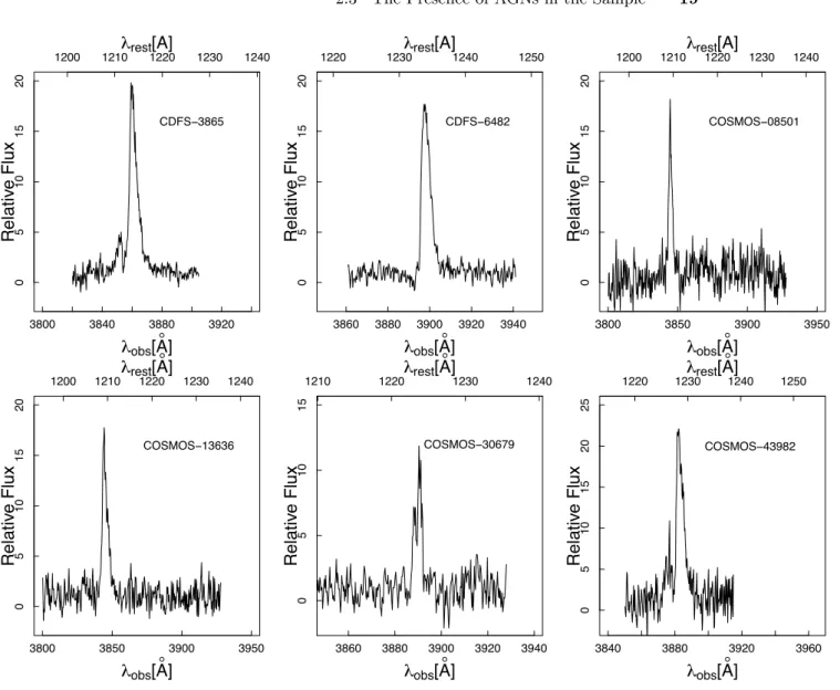
The spectra were reduced with IDL based pipeline, MagE REDUCE, constructed by G. Becker (see also Kelson 2003). This pipeline processes the raw frames, performing the wavelength calibration, optimal sky subtraction, and extracts their 1D spectrum. Each of these reduced frames was then combined to form our final calibrated spectrum. We inspect one order of the echelle spectra ranging from 3520 ˚A to 4100 ˚A in the observed frame, which covers a Lyα line. From this, a Lyα line was identified above the 3 σ noise of the local continuum.

The calibrated 1D spectra are shown in Figure 2.3, where y− axis is the relative flux. This is due to the fact that echelle spectra are notorious for flux-calibration.

2.2.2 LRIS Spectroscopy and Reduction

The four COSMOS objects and two SXDS objects, COSMOS-08357, COSMOS-12085, COSMOS-13138, COSMOS-38380, SXDS-10600, and SXDS-10942, were observed with LRIS on the Keck I telescope on 2012 March 19 – 21 and November 14 – 15. Details of the observation and data reduction procedures are presented in Shibuya et al. (2014a). Briefly, the objects were observed with the 600/500 gratings, whose spectral coverage and spectral resolution are 3300˚A – 5880˚A and R ∼ 1000, respectively. The seeing size was 0.′′_{7 – 1.}′′_6.

We identified a Lyα line in all of the objects. In addition, we detected several metal absorption lines (e.g., Si ii λ1260 and Civ λ1548 lines) in individual LRIS spectra of COSMOS-12805, COSMOS-13636, and SXDS-10600 (Shibuya et al. 2014a).

(35)

3800 3840 3880 3920 0 5 10 15 20 CDFS−3865 λobs[A° ] Relativ e Flux 3860 3880 3900 3920 3940 0 5 10 15 20 CDFS−6482 λobs[A° ] Relativ e Flux 3800 3850 3900 3950 0 5 10 15 20 COSMOS−08501 λobs[A° ] Relativ e Flux 3800 3850 3900 3950 0 5 10 15 20 COSMOS−13636 λobs[A° ] λrest[A° ] Relativ e Flux 1200 1210 1220 1230 1240 3860 3880 3900 3920 3940 0 5 10 15 COSMOS−30679 λobs[A° ] λrest[A° ] Relativ e Flux 1210 1220 1230 1240 3840 3880 3920 3960 0 5 10 15 20 25 COSMOS−43982 λobs[A° ] λrest[A° ] Relativ e Flux 1220 1230 1240 1250

Figure 2.3. Reduced 1D spectra taken by MagE.

Lyα line is denoted by the red dotted line.

A summary of our observations is listed in Table 2.1.

2.3 The Presence of AGNs in the Sample

The presence of AGNs in the MagE objects has been examined in Hashimoto et al. (2013) and Nakajima et al. (2013), and those of the LRIS objects in Shibuya et al. (2014a). In short, for the MagE objects, we inspected it in three ways. We first compared the sky coordinates of the objects with those in very deep archival X-ray and radio catalogs. Then we checked for the presence of high ionization state lines such as Civ λ 1549 and He ii λ1640 lines in the spectra. Finally, we applied the BPT diagnostic diagram (Baldwin et al. 1981) to the objects. An AGN activity is not seen in the objects except for

(36)

COSMOS-3800 4000 4200 4400 4600 4800 5000 5200 0 5 10 COSMOS−08357 λobs[A° ] λrest[A° ] Relativ e Flux 1200 1300 1400 1500 1600 3800 4000 4200 4400 4600 4800 5000 5200 0 2 4 6 8 10 12 COSMOS−12805 λobs[A° ] λrest[A° ] Relativ e Flux 1200 1300 1400 1500 1600 3800 4000 4200 4400 4600 4800 5000 5200 0 5 10 15 20 COSMOS−13138 λobs[A° ] λrest[A° ] Relativ e Flux 1200 1300 1400 1500 1600 3800 4000 4200 4400 4600 4800 5000 5200 0 5 10 15 20 COSMOS−13636 λobs[A° ] λrest[A° ] Relativ e Flux 1200 1300 1400 1500 1600 3800 4000 4200 4400 4600 4800 5000 5200 0 10 20 30 40 50 COSMOS−38380 λobs[A° ] λrest[A° ] Relativ e Flux 1200 1300 1400 1500 1600 3800 4000 4200 4400 4600 4800 5000 5200 0 5 10 15 20 COSMOS−43982 λobs[A° ] λrest[A° ] Relativ e Flux 1200 1300 1400 1500 1600 3800 4000 4200 4400 4600 4800 5000 5200 0 5 10 15 20 25 30 SXDS−10600 λobs[A° ] λrest[A° ] Relativ e Flux 1200 1300 1400 1500 1600 3800 4000 4200 4400 4600 4800 5000 5200 0 10 20 30 40 50 SXDS−10942 λobs[A° ] λrest[A° ] Relativ e Flux 1200 1300 1400 1500 1600

Figure 2.4. Reduced 1D spectra taken by LRIS. The red dotted line corresponds to the Lyα wavelength.

(37)

On the other hand, due to a lack of Hα or [Nii] λ6568 data, we were only able to use the two forms of investigation for the LRIS objects. Of these, only COSMOS-43982 showed clear detection of a Civ λ 1549 line in its optical spectrum.

In summary, we have ruled out AGN activity in all sample’s objects, except for COSMOS-43982.

(38)

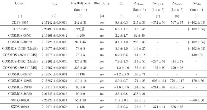
Table 2.1. Summary of our observations

Object α(J2000) δ(J2000) EW(Lyα)photo L(Lyα) NIR obs. opt. obs. Sourcea

(˚A) (1042_{erg s}−1₎ ₍₁₎

(2) (3) (4) (5) (6) (7) (8)

CDFS-3865 03:32:32.31 -28:00:52.20 64 ± 29 29.8 ± 4.9 NIRSPEC (J) MagE H13, N13

MMIRS (HK)

CDFS-6482 03:32:49.34 -27:59:52.35 76 ± 52 15.4 ± 8.1 MMIRS (HK) MagE H13, N13

COSMOS-08501 10:01:16.80 +02:05:36.26 280 ± 30 8.8 ± 1.1 NIRESPC (K) MagE N13

COSMOS-30679 10:00:29.81 +02:18:49.00 87 ± 7 8.5 ± 0.7 NIRSPEC (H and K) MagE H13, N13

COSMOS-13636 09:59:59.38 +02:08:38.36 73 ± 5 11.3 ± 0.5 FMOS (H) MagE and LRIS H13, N13, S14

NIRSPEC (K)

COSMOS-43982b _{09:59:54.39 +02:26:29.96} _{130 ± 12} _{11.0 ± 0.5} _{MMIRS (HK)} _{MagE and LRIS H13, N13, S14}

COSMOS-08357 09:59:59.07 +02:05:31.60 47 ± 8 0.5 ± 0.1 FMOS (H) LRIS S14, N14b

SXDS-10600 02:17:46.09 -06:57:05.00 58 ± 3 1.9 ± 0.1 FMOS (H) LRIS S14, N14b

SXDS-10942 02:17:59.54 -06:57:25.60 135 ± 10 0.3 ± 0.0 FMOS (H) LRIS S14, N14b

Notes.— (1) Object ID; (2)(3) Right ascension and Declination; (4)(5) rest-frame Lyα EW and lumi-nosity derived from narrow- and broadband photometry; (6) Instruments and filters used for the NIR observations; (7) Instruments used for the optical observations; and (8) source of the information a – H13: Hashimoto et al. (2013); N13: Nakajima et al. (2013); S14: Shibuya et al. (2014a); N14b: Nakajima et al (2014, in preparation) b – AGN-like object

(39)

Chapter 3

Observational Results

3.1 Spectroscopic Properties

3.1.1 Line Centroid and FWHM Measurements for Nebular Emission Lines

Line centroid (i.e., redshift) and FWHM measurements of nebular emission lines are crucial for a detailed modeling of the Lyα line, since they encode information on the intrinsic (i.e., before being aﬀected by radiative transfer) Lyα redshift and FWHM. In order to obtain these parameters and their uncertainties, we apply a Monte Carlo technique as follows. First, for each object and for each line, we measure the 1σ noise of the local continuum. Then we create 103 _{fake spectra by perturbing the flux at each wavelength of the true}

spectrum by the measured 1σ error (Kulas et al. 2012; Chonis et al. 2013). For each fake spectrum, the wavelength at the highest flux peak is adopted as the line centroid, and the wavelength range encompassing half the maximum flux is adopted as the FWHM. The standard deviation of the distribution of measurements from the 103 _{artificial spectra is}

adopted as the error on the line centroid and FWHM. When multiple lines are detected, we adopt a weighted mean value of them. A summary of the measurements are listed in columns 2 and 3 of Table 3.1. All redshift (FWHM) values are corrected for the LSR motion (instrumental resolution). When the line is unresolved, the instrumental resolution is given as an upper limit. The mean FWHM value for the sample of 8 objects with a measurable velocity dispersion is FWHM(neb) = 129 ± 55 km−1_{, which is smaller than}

that of LBGs, FWHM(neb) = 200−250 km−1_{(Pettini et al. 2001; Erb et al. 2006a; Kulas}

et al. 2012). This is consistent with the recent results of Erb et al. (2014), who have found that the median FWHM(neb) in 36 z ∼ 2 LAEs is 127 km s−1_{. These results indicate}

(40)

Table 3.1. Summary of the spectroscopic properties of the sample

Object zsys FWHM(neb) Blue Bump Sw ∆vLyα,r ∆vLyα,b ∆vpeak ∆vabs

(km s−1₎ _{(km s}−1₎ _{(km s}−1₎ _{(km s}−1₎ _{(km s}−1₎ (1) (2) (3) (4) (5) (6) (7) (8) (9) CDFS-3865 2.17242 ± 0.00016 242 ± 31 yes 8.8 ± 0.3 245 ± 36 −352 ± 59 597 ± 67 (−102 ± 65) CDFS-6482 2.20490 ± 0.00042 99+66 −99 no 6.6 ± 1.7 118 ± 48 - - (−102 ± 65) COSMOS-08501 2.16161 ± 0.00042 < 200 no 2.2 ± 2.7 82 ± 40 - -COSMOS-30679 2.19725 ± 0.00020 92 ± 45 no 3.1 ± 1.0 290 ± 33 - - (−102 ± 65) COSMOS-13636 (MagE) 2.16075 ± 0.00019 73 ± 5 no 5.3 ± 1.0 146 ± 25 - - (−102 ± 65) COSMOS-13636 (LRIS) 2.16075 ± 0.00019 73 ± 5 no 6.2 ± 0.5 161 ± 18 - - -130±70

COSMOS-43982 (MagE) 2.19267 ± 0.00036 325 ± 36 yes 7.9 ± 1.3 117 ± 53 −297 ± 57 414 ± 78

-COSMOS-43982 (LRIS) 2.19267 ± 0.00036 325 ± 36 yes −4.2 ± 0.6 155 ± 40 −165 ± 90 320 ± 98

-COSMOS-08357 2.18053 ± 0.00031 < 136 no −4.2 ± 7.9 106 ± 71 - - -COSMOS-12805 2.15887 ± 0.00024 110 ± 16 yes 8.9 ± 0.7 171 ± 25 −605 ± 114 776 ± 117 −170 ± 50 COSMOS-13138 2.17914 ± 0.00012 63 ± 6 yes −1.6 ± 4.8 191 ± 59 −214 ± 87 405 ± 105 -COSMOS-38380 2.21245 ± 0.00015 99 ± 9 no 2.5 ± 0.8 338 ± 21 - - -SXDS-10600 2.20922 ± 0.00014 55 ± 28 no 11.7 ± 0.2 186 ± 13 - - −260 ± 60 SXDS-10942 2.19574 ± 0.00025 < 136 yes 1.3 ± 0.3 135 ± 10 −374 ± 41 556 ± 66

-Notes.— The symbol “-” indicates we have no measurement. (1) Object ID; (2) Systemic redshift derived from the weighted mean of the nebular emission redshifts; (3) Weighted mean FWHM of nebular emission line; (4) Presence of the blue bump emission in the Lyα profile; (5) Weighted skewness of the Lyα line

(Kashikawa et al. 2006); (6) Velocity oﬀset of the Lyα main red peak with respect to the zsys; (7) Velocity

oﬀset of the Lyα blue-bump with respect to the zsys; (8) Peaks separation between ∆vLyα,rand ∆vLyα,b;

and (9) Mean velocity oﬀset of LIS absorption lines with respect to the zsys (Hashimoto et al. 2013;

Shibuya et al. 2014a).

3.1.2 Lyα Profiles

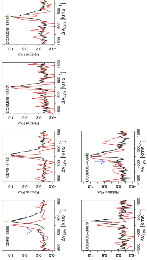
While the majority of Lyα profiles are single-peaked (e.g., Shapley et al. 2003; Steidel et al. 2010), a fraction of Lyα profiles are known to be multiple-peaked (e.g., Yamada et al. 2012; Kulas et al. 2012). In particular, a secondary small peak blueward of the systemic redshift is called a “blue bump” (see the case 2 profile in Figure 12 in Verhamme et al. 2006). Theoretical studies have shown that the blue bump is a natural outcome of the radiative transfer in a low speed galactic outflow (e.g., Zheng & Miralda-Escud´e 2002).

(41)

detect blue emission in five objects and in six spectra; MagE ones of CDFS-3865 and COSMOS-43982, and LRIS ones of COSMOS-12805, COSMOS-13138, COSMOS-43982, and SXDS-10942. From the fact that these spectra show a main red peak with a secondary blue peak, we conclude that these spectra have a blue bump. The position of the blue bump is designated by a blue arrow in Figures 3.1 and 3.2, where both Lyα and nebular lines are converted into the velocity space. The velocity zero point in these figures is determined by the systemic redshift. The result is summarized in the column 4 of Table 3.1.

The frequency of blue bump objects in the sample is ∼ 40% (5/12). There are four LAEs in the literature that have a blue bump: one among the two LAEs studied in McLinden et al. (2011) and all three LAEs studied in Chonis et al. (2013). For a total sample of 17 LAEs, the frequency is calculated to be ∼ 50% (9/17). Note that this is a lower limit due to the limited spectral resolution. On the other hand, Kulas et al. (2012) have studied 18 z_{∼ 2 − 3 LBGs with z}sys measurements which are preselected to have a multiple-peaked

Lyα profile. They have argued that ∼ 30% of the parent sample are multiple-peaked and that 11 out of the 18 objects have a blue bump, indicating that the blue bump frequency in LBGs is ∼ 20% (∼ 30% × 11/18). These results imply that the blue bump feature is slightly more common in LAEs than in LBGs. However, a larger sample, observed at a higher spectral resolution, is needed for a definite conclusion.

Observed Lyα lines usually have an asymmetric profile with a red tail and a sharp blue cut oﬀ. Some studies at high-z utilize the asymmetry of the Lyα line to distinguish it from interloper lines of foreground galaxies. Thanks to the simultaneous detection of Lyα and nebular emission lines, it is no doubt that our detected lines are Lyα lines. Still, it is useful to quantify the asymmetry of the Lyα line of our objects. We use the weighted skewness, Sw (Kashikawa et al., 2006). Skewness is the third moment of the flux

distribution, and the weighted skewness is defined as the product of the skewness and the line width. A positive Sw means that the Lyα profile has a red tail. The measured Sw

values for the sample are listed in the column 5 of Table 3.1. While most spectra have a positive Sw value beyond the 1 σ uncertainty, four spectra, MagE-COSMOS-08501,

LRIS-COSMOS-08357, LRIS-COSMOS-43982, and LRIS-COSMOS-13138, have Sw ∼ 0

]

COSMOS − 43982

Figure 3.1. Lyα lines obtained by MagE (black) and Hα lines obtained by MMIRS or NIRSPEC (red), All spectra are scaled in the wavelength range from −1500 to +1500 km s−1. Green and orange segments indicate the peak flux positions derived from a Gaussian and a Monte Carlo techniques, respectively.

− 1

]

SXDS − 10600 −0.2 0.2 0.6 1.0 −1500 − 500 500 1500 −0.2 0.2 0.6 1.0 Relative Flux

∆

v

Ly α

[km

s

− 1

]

SXDS − 10942

Figure 3.2. Lyα lines obtained by LRIS (black) and [Oiii] lines by FMOS (red), All spectra are scaled in the wavelength range from −1500 to +1500 km s−1. The meanings of the two segments are the same as those in Figure 3.1.2.

(44)

3.1.3 Lyα Velocity Properties

We derive three velocity oﬀsets related to the Lyα line: the velocity oﬀset of the main red peak of the Lyα line with respect to the systemic,

∆vLyα,r= c

zLyα,r− zsys

1 + zsys

, (3.1)

; that of the blue bump of a Lyα line with respect to the systemic, if any,

∆vLyα,b= c

zLyα,b− zsys

1 + zsys

, (3.2)

; and that of the two peaks,

∆vpeak= ∆vLyα,r− ∆vLyα,b, (3.3)

where zsys, zLyα,r, and zLyα,brepresent the systemic redshift, the Lyα redshift of the main

red peak, and that of the blue bump, respectively. Lyα Main Red Peak Velocity Oﬀsets, ∆vLyα,r

We estimate the ∆vLyα,r value using a Monte Carlo technique in a similar manner to

that in §3.1.1. First, for each object, we measure a 1σ error of the Lyα spectrum set by the continuum level at the wavelength longer than 1216˚A. Then we create 103 _fake

spectra converted into the velocity space by simultaneously perturbing the flux at each wavelength and the systemic redshift listed in Table 3.1 by their 1σ errors. Finally, we measure the velocity at the highest flux peak. The mean and the standard deviation value of the distribution of 103 _{measurements is adopted as the ∆v}

Lyα,r and its error,

respectively. The derived ∆vLyα,r values are listed in the column 6 of Table 3.1, ranging

from 82 km s−1_{to 338 km s}−1_{with a mean value of 174 ±19 km s}−1_{. In most cases, these}

values are consistent with those measured in Hashimoto et al. (2013) and Shibuya et al. (2014a) within 1σ, however, they are not for COSMOS-08357 and COSMOS-12805. This is due to the fact that these studies have applied a symmetric/asymmetric profile fit to the Lyα line. In Figures 3.1 and 3.2, we show the two ∆vLyα,r values derived from the Monte

Carlo and the profile fit technique as the green and orange line segments, respectively. For the sake of consistency in the definition of the ∆vLyα,r in the shell model (Verhamme

et al. 2006; Schaerer et al. 2011), we adopt these new measurements. We note that our discussions remain unchanged even if we adopt previous ∆vLyα,r values.

The ∆vLyα,r value has been measured in more than 60 LAEs (McLinden et al. 2011;

Lyαスペクトルで探る遠方星形成銀河のアウトフロー

Outflows in Distant Star Forming Galaxies

Probed by Lyman Alpha Spectra

(

Ly

αスペクトルで探る遠方星形成銀河のアウトフロー

)

Takuya Hashimoto

橋本 拓也

東京大学大学院理学系研究科天文学専攻

平成２６年１２月 博士（理学）申請

Outflows in Distant Star Forming Galaxies

Probed by Lyman Alpha Spectra

(

Ly

αスペクトルで探る遠方星形成銀河のアウトフロー

)

35-127074

Takuya Hashimoto

橋本 拓也

Department of Astronomy, Graduate School of Science

The University of Tokyo

Abstract

Contents

List of Figures

List of Tables

Chapter 1

Introduction

1.1 Galaxies

1.2 High-Redshift Galaxies

1.2.1 Lyman Break Galaxies

1.2.2 Lyman Alpha Emitters

1.3 Previous Studies Related to LAEs

1.3.1 Clustering Analysis of LAEs

1.3.2 LAEs as a Probe of Cosmic Reionization

1.3.3 Recent Findings of LAEs

1.4 Open Questions concerning LAEs

1.4.1 The Presence of Outflows

1.4.2 The Lyα Escape Mechanism

1.5 Open Questions Concerning Cosmic Reionization

1.6 Goals of This Thesis

Chapter 2

Observations & Data

2.1 Near-Infrared Spectroscopy

2.1.1 MMIRS Spectroscopy and Reduction

2.1.2 NIRSPEC Spectroscopy and Reduction

2.1.3 FMOS Spectroscopy and Reduction

2.2 Optical Spectroscopy

2.2.1 MagE Spectroscopy and Reduction

2.2.2 LRIS Spectroscopy and Reduction

2.3 The Presence of AGNs in the Sample

Chapter 3

Observational Results

3.1 Spectroscopic Properties

3.1.1 Line Centroid and FWHM Measurements for Nebular Emission Lines

3.1.2 Lyα Profiles

∆

v

[km

s

]

∆

v

[km

s

]

∆

v

[km

s

]

∆

v

[km

s

]

∆

v

[km

s

橋本拓也

　　　　　東京大学大学院理学系研究科天文学専攻

平成２６年１２月　博士（理学）申請

橋本拓也