Singular value decomposition for a class of
linear time-varying systems with application
to switched linear systems
著者
Hara Naoyuki, Kokame Hideki, Konishi Keiji
journal or
publication title
Systems & Control Letters
volume
59
number
12
page range
792-798
year
2010-12
権利
c2010 Elsevier B.V. All rights reserved
URL
http://hdl.handle.net/10466/12518
Singular value decomposition for a class of linear
time-varying systems with application to switched linear
systems
N. Hara1,∗, H. Kokame1, K. Konishi1
Department of Electrical and Information Systems, Osaka Prefecture University, Osaka 599-8531, Japan.
Abstract
The present paper considers singular value decomposition (SVD) for a class of linear varying systems. The class considered herein describes time-driven switched linear systems. Based on an appropriate input-output de-scription, the calculation method of singular values and singular vectors is derived. The SVD enables us to characterize the dominant input–output sig-nals using singular vectors, which form orthogonal systems in input and out-put spaces. The SVD is then applied to switched linear systems to improve the transient response. A numerical example is provided to demonstrate the proposed method.
Keywords: Singular value decomposition, switched linear system, feedforward compensation, linear operator.
1. Introduction
For linear dynamical systems, singular value decomposition (SVD) plays an important role in analysis and control, and SVD has been investigated in a number of studies. For example, model reduction methods for finite-dimensional linear systems have been developed [1, Chapters 7 and 8], and the finite-dimensional approximation problem of a class of infinite-dimensional
∗Corresponding author: N. Hara: Tel:+81-72-254-9252, Fax:+81-72-254-9907
Email addresses: [email protected] (N. Hara),
systems has been considered [2]. Exact formulas for singular values and vec-tors of a system consisting of an SISO inner function and an MIMO rational function have been derived [3]. A compensation signal design method for improving the transient response of linear systems has been derived based on the SVD for linear time-invariant systems [4]. For constrained systems, the compensation signal design problem has been reported [5]. Model pre-dictive control for constrained continuous-time linear systems has also been developed [6]. In these recent studies, singular vectors serve as effective basis vectors for generating approximate continuous-time signals in infinite dimen-sional function spaces. If the formulas for calculating the singular values and singular vectors for a suitably defined system of interest can be established, SVD-based methods might be applied to various control and approximation problems.
In the present paper, we first consider the SVD of an operator describ-ing the input-output relation of a class of linear time-varydescrib-ing systems and derive a method for calculating singular values and singular vectors. The SVD provides orthogonal input and output sequences that enable us to ap-proximate the original infinite-dimensional input and output spaces using a finite number of singular vectors. The class of systems considered herein represents time-driven switched linear systems, and we consider the com-pensation signal design problem for switched linear systems with a periodic switching law to improve the transient response using the newly established SVD. The compensation signal design we consider in the present paper is based on a feedforward method and the resulting compensation input over the entire time interval of interest is computed off-line using the desired and uncompensated responses.
The remainder of the present paper is organized as follows. In Section 2, the SVD of an operator describing a class of linear time-varying systems is considered, and the calculation method of singular values and singular vectors is derived. In Section 3, the obtained SVD is applied to a switched linear system with a periodic switching law, and the compensation law for improving the transient response is considered. A numerical example is pre-sented in Section 4 to illustrate the fundamental properties of the proposed method.
2. Singular Value Decomposition for a Class of Linear Time-varying Systems
Consider a class of linear time-varying systems defined over a finite hori-zon [0, h]: Σ : { ˙x(t) = A(t)x(t) + B(t)v(t), x(0) = 0 z(t) = E(t)x(t) (1) (A(t), B(t), E(t)) := (A1, B1, E1) 0≤ t < t1 (A2, B2, E2) t1 ≤ t < t2 .. . ... (AN, BN, EN) tN−1 ≤ t ≤ tN t0 = 0 < t1 < t2 <· · · < tN = h
where x(t) ∈ Rnx, v(t) ∈ Rnv, and z(t) ∈ Rnz denote the state, input,
and output, respectively. This system represents a time-dependent switched linear system. Switched linear systems with a periodic switching law can be described by this particular form (additional details are presented in Section 3). In this section, starting with the introduction of appropriate generalized input and output spaces, we derive the singular value decomposition method for the system given in (1), which will be used for the transient improvement of switched linear systems.
First, define Hilbert spacesV := L2(0, h;Rnv) andZ := Rnx×L2(0, h;Rnz)
with the inner products
⟨f1, f2⟩V := ∫ h 0 f1T(β)f2(β)dβ, f1, f2 ∈ V, (2) ⟨g1, g2⟩Z := g0 T 1 g 0 2+ ∫ h 0 g11T(β)g12(β)dβ, g1 = [ g10 g1 1 ] , g2 = [ g20 g1 2 ] ∈ Z (3)
and denote the input and output in V and Z as
v ∈ V, ˆz := [ z0 z1 ] ∈ Z, z0 := F x(h), F ∈ Rnx×nx, (4) z1(t) := z(t), 0≤ t ≤ h
where F is a weighting matrix for the terminal state. The relationship be-tween v and ˆz is given by a linear operator Γ∈ L(V, Z):
ˆ z = Γv Γv := [ (Γv)0 (Γv)1 ] , (Γv)0 =F N∑−1 s=1 Φ(N,s)(h) ∫ ts ts−1 eAs(ts−τ)B sv(τ )dτ + F ∫ h tN−1 eAN(h−τ)B Nv(τ )dτ, (5) (Γv)1[t k,tk+1](t) =Ek+1 k ∑ s=1 Φ(k+1,s)(t) ∫ ts ts−1 eAs(ts−τ)B sv(τ )dτ + Ek+1 ∫ t tk eAk+1(t−τ)B k+1v(τ )dτ, (6) tk≤ t ≤ tk+1, k = 0, . . . , N − 1, Φ(ℓ,m)(t) :=eAℓ(t−tℓ−1)eAℓ−1(tℓ−1−tℓ−2)· · · eAm+1(tm+1−tm), ℓ, m∈ Z+ : ℓ > m≥ 0, tℓ−1 ≤ t ≤ tℓ.
Note that (Γv)0 and (Γv)1 denote the weighted terminal state and output
signal corresponding to the input signal v over [0, h], respectively. For the operator Γ, we consider the following singular value problem:
Γf = σg, Γ∗g = σf, (7)
σ∈ R, f ∈ V, g ∈ Z, (f ̸= 0, g ̸= 0).
The singular vectors f and g represent the input and output signals inV and
Z. The pairs (f, g) corresponding to the larger singular values σ characterize
the dominant input–output behavior of the system Σ. The following theo-rem provides a calculation method of the singular values σ and the explicit characterization of the singular vectors f and g that satisfy the relation (7).
transcendental equation: det{M(σ)} = 0, (8) M (σ) :=[−σ1FTF I]eJN(σ) ¯dNeJN−1(σ) ¯dN−1· · · eJ1(σ) ¯d1 [ 0 I ] , Jm(σ) := [ Am σ1BmBmT −1 σE T mEm −ATm ] , ¯dm := tm− tm−1, m = 1, 2, . . . , N.
Let σi be a singular value. Then, the corresponding singular vectors fi ∈ V
and gi ∈ Z are given as follows:
fi[tk−1,tk](β) = 1 σi [ 0 BkT]eJk(σi)(β−tk−1)eJk−1(σi) ¯dk−1· · · eJ1(σi) ¯d1 [ 0 I ] qi, k = 1, 2, . . . , N, (9) gi0 = 1 σi [ F 0]eJN(σi) ¯dNeJN−1(σi) ¯dN−1· · · eJ1(σi) ¯d1 [ 0 I ] qi, (10) gi [t1 k−1,tk](β) = 1 σi [ Ek 0 ] eJk(σi)(β−tk−1)eJk−1(σi) ¯dk−1· · · eJ1(σi) ¯d1 [ 0 I ] qi, k = 1, 2, . . . , N, (11) qi ̸= 0 : M(σi)qi = 0.
Proof. For the operator Γ , the adjoint Γ∗ ∈ L(Z, V) is calculated as follows
(see the Appendix for details):
(Γ∗z)ˆ [tk−1,tk](τ ) = BkTeAkT(tk−τ)ΦT (N,k)(h)F Tzˆ0 + N∑−1 s=k ∫ ts+1 ts BkTeAkT(tk−τ)ΦT (s+1,k)(β)E T kzˆ 1(β)dβ + ∫ tk τ BkTeAkT(β−τ)ET kzˆ 1(β)dβ tk−1 ≤ τ ≤ tk, k = 1, 2, . . . , N− 1, BNTeANT(h−τ)FTzˆ0+ ∫ tN τ BNTeANT(β−τ)ET Nzˆ 1 (β)dβ tN−1 ≤ τ ≤ tN, k = N (12) ˆ z = [ ˆ z0 ˆ z1 ] ∈ Z.
By introducing the auxiliary variables p1(t) := ∫ t 0 eA1(t−τ)B 1v(τ )dτ, 0≤ t ≤ t1, pk(t) := eAk(t−tk−1)pk−1(tk−1) + ∫ t tk−1 eAk(t−τ)B kv(τ )dτ, tk−1 ≤ t ≤ tk, k = 2, 3, . . . , N, qN(t) := eA T N(tN−t)FTzˆ0+ ∫ tN t eATN(β−t)ET Nzˆ 1(β)dβ, qk(t) := eA T k(tk−t)q k+1(tk) + ∫ tk t eATk(β−t)ET kzˆ 1(β)dβ, tk−1 ≤ t ≤ tk, k = 1, 2, . . . , N − 1
to (5), (6), and (12), the relation (7) is rewritten as the following set of equations: ˙ pk(t) = Akpk(t) + Bkv(t), (13) σ ˆz1(t) = Ekpk(t), (14) tk−1 ≤ t ≤ tk, k = 1, 2, . . . , N, σ ˆz0 = F pN(tN), (15) p1(0) = 0, (16) ˙ qk(t) =−ATkqk(t)− EkTzˆ1(t), (17) tk−1 ≤ t ≤ tk, k = 1, 2, . . . , N, σv(t) = BkTqk(t), (18) qN(tN) = FTzˆ0. (19)
By eliminating v and ˆz1 from the differential equations (13) and (17) using
(14) and (18), (13) and (17) yield the following differential equation: [ ˙ pk(t) ˙ qk(t) ] = [ Ak σ1BkBkT −1 σE T kEk −ATk ] [ pk(t) qk(t) ] .
The solution to this differential equation on [tk−1, tk] is given by [ pk(tk) qk(tk) ] = eJk(σ)(tk−tk−1) [ pk−1(tk−1) qk−1(tk−1) ] .
From equations (15) and (19), the boundary condition qN(tN) = 1σFTF pN(tN), which implies [−1 σF TF, I] [ pN(h) qN(h) ] = 0, is obtained. Then, we have
[ −1 σF TF I] [pN(h) qN(h) ] =[−1σFTF I]eJN(σ) ¯dN [ pN−1(tN−1) qN−1(tN−1) ] =· · · =[−1σFTF I]eJN(σ) ¯dNeJN−1(σ) ¯dN−1· · · eJ1(σ) ¯d1 [ 0 I ] q1(0) = M (σ)q1(0) = 0. (20)
Since it has been shown that q1(0) ̸= 0 iff f ̸= 0, and g ̸= 0, the matrix M (σ) in (20) must be singular for the singular value σ. Therefore, the singular values are given by the roots of equation (8). The singular vectors (9) through (11) corresponding to the singular value σ are constructed by expressing v, z0, and z1 using the auxiliary variables p
k and qk.
Remark 2. The singular vectors{fi}, and {gi} form orthogonal sequences in
spaces V and Z. The singular vectors fi corresponding to the large singular
values describe the input signals over [0, h] that have a significant effect on the input-output dynamics of the linear time-varying system (1) because the output ˆz is given as σi· gi, which indicates that the output gi is multiplied by
σi when fi is applied to the system.
Remark 3. The singular values are calculated by using general methods such as the bisection algorithm. Once the singular values are calculated from the determinant equation (8), the singular vectors are easily computed from (9) through (11) because they have the form of the autonomous response of a switched linear system. Although there are infinitely many discrete singular values, which approaches zero, we use only larger singular values and the
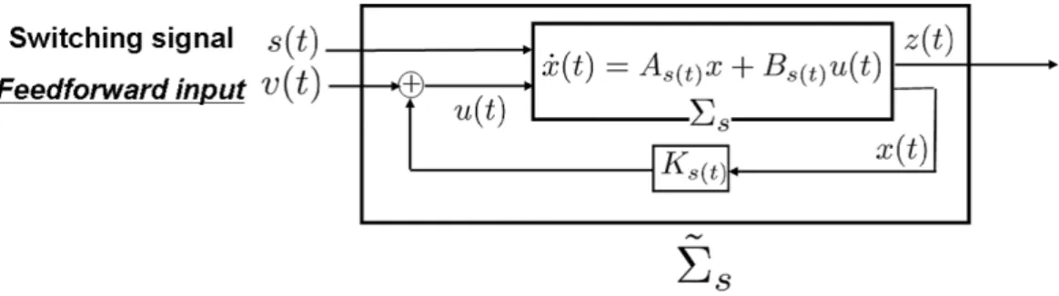
Figure 1: Switched linear system with compensation.
corresponding singular vectors in the compensation design. When a singular value σi is found from (8), it may be necessary to check whether σi is the
largest root. In [7], the method for counting the zeros (roots) for a similar type of equation on a given interval has been considered based on a winding number method in complex analysis. This approach is also applicable to the present case.
Based on the SVD for switched linear systems obtained in this section, we derive a feedforward compensation signal design method for switched linear systems.
In the following, we normalize the singular vectors as∥fi∥V = 1,∥gi∥Z = 1 and denote the singular values by σ1 ≥ σ2 ≥ σ3 ≥ · · · in decreasing order
and the corresponding singular vectors by fi and gi (i = 1, 2, . . . ).
3. Transient Improvement for a Switched Linear System with Pe-riodic Switching
A switched system consists of several subsystems and a switching sig-nal that determines the transition of the dynamics among the subsystems. The stabilizing switching law, system structures (controllability and observ-ability), and optimal control have been investigated in a number of studies [8, 9, 10, 11, 12, 13].
From practical viewpoint, there are many systems which are formulated as switched systems. In addition, some control problems can be formulated in the framework of switched systems, e.g., multi-controller scheme for systems with large uncertainty (see, for example, [8, 10, 14]). A typical example of a
switched system is an electronic circuit with an on-off switch realized using transistor (e.g., DC-DC converter). In this system, the on-off switch acts as a discrete switching signal, which corresponds to switch the subsystem, and a voltage (or current) input signal corresponds to a continuous-time input signal. A simple model of a manual transmission is also an example of switched systems, where the gear shift position is a discrete-valued input and the input acceleration is a continuous-time signal [15]. Two distinctive switching laws for switched systems are the time-driven switching law and the even-driven (state-dependent) switching law, and various switching laws have been proposed so far [8]. When the event-driven switching law is applied to a switched system, the resulting system is considered as a hybrid system whose dynamics changes depending on the value of the state. In the case of the dependent switching law, the resultant system is considered as a time-varying system. In the control of these systems, the relationship between the switching of subsystems and continuous-time signal has to be taken into account to design control inputs. The SVD considered in the previous section provides a way to clarify this relationship for, in particular, switched linear systems with the time-driven switching law.
In the optimal control of the switched systems, the optimal design of both the switching signal and continuous-time input is by nature a difficult problem [8]. Moreover, if one pursues optimality exclusively, the switch-ing frequency might become very high or the switchswitch-ing law might require infinitely many switchings on a finite interval [12, 13], which is not desir-able from a practical viewpoint. Instead of designing the switching signal to achieve good performance, we consider the feedforward compensation signal design problem.
In this section, based on the SVD for the class of linear time-varying sys-tems developed in the previous section, we derive a method for improving the transient response of a switched linear system with a periodic switching law. The compensation signal is computed off-line beforehand based on un-compensated and desired transient response over the finite time interval of interest.
First, we consider the following switched linear system: Σs :
{
˙x(t) = As(t)x(t) + Bs(t)u(t)
z(t) = Es(t)x(t)
(21) where x(t), u(t), and z(t) denote the state, input, and output, respectively. Subscript s(t) ∈ S := {1, 2, . . . , r} denotes the switching signal, where r is
the number of the subsystems. When we apply
u(t) = Ks(t)x(t) + v(t) (22)
to Σs, the resulting system ˜Σs (Fig. 1) is described by ˜ Σs: { ˙x(t) = ˜As(t)x(t) + Bs(t)v(t) z(t) = Es(t)x(t) ˜ As(t) := As(t)+ Bs(t)Ks(t).
In (22), v(t) denotes the compensation signal that we will design to improve the transient response. If feedback gain matrices Ki and coefficients ωi exist such that the following convex combination of ˜Ai is Hurwitz:
A0 = ∑ i∈S wiA˜i (ωi ≥ 0, ∑ i∈S ωi = 1), (23)
then the system can be stabilized via periodic switching signal as follows [8, 9]. Let Ki and wi be one pair that satisfies (23). Then, for a small T > 0, the periodic switching signal
s(t) = 1, t∈ [kT, (k + ω1)T ) 2, t∈ [(k + ω1)T, (k + ω1+ ω2)T ) .. . ... r, t∈ [(k + 1 − ωr)T, (k + 1)T ) k = 0, 1, . . .
stabilizes the system exponentially because matrix Ad:= eωrArT · · · eω1A1T =
eA0T +f (T )T2 (f is an analytic and bounded matrix-valued function) can be stable for T > 0, and x((k + 1)T ) = Adx(kT ) holds. Consequently, a system with the periodic switching signal can be represented in the form of the lin-ear time-varying system (1). Note that the switching interval of the above switching law is given by ωi· T . If the lower limit Tlow > 0 for the switching interval is imposed, one needs to pay attention to the choice of ωi and T so that the condition ωi · T ≥ Tlow is satisfied. From the implementation viewpoint, the switching control law is relatively simple because of its pe-riodicity, and it is especially applicable to the systems where the switching rule cannot be arbitrarily modified during operation due to limitations on hardware and/or software.
For the system stabilized by the periodic switching signal, we consider the transient improvement by the compensation input v(t) over the finite horizon 0 ≤ t ≤ h in the sense that the resulting system response approaches a certain prescribed response. Let
ˆ yd = [ xd(h) yd[0,h] ] ∈ Z
be a desired output in Z (pair of the terminal state and the output signal), and let ˆ y = [ x(h) y[0,h] ] ∈ Z
be the nominal response (without compensation input v). The desired re-sponse ˆyd can be chosen from the response of a certain reference model that has a good transient property. Define the error ˆe := ˆyd− ˆy ∈ Z. We de-sign compensation input v(t) such that the resulting system response closely approximates the desired response ˆyd. We construct the compensation input
v(t) by the linear combination of the singular vectors fi ∈ V corresponding to Ns> 0 singular values in decreasing order, which represent the dominant input signals over [0, h] in V. Since Ns singular vectors g1, g2, . . . , gNs form
the orthonormal system in Z, the closest element of span{g1, g2, . . . , gNs} to
ˆ e is given by ˆ e′ := Ns ∑ i=1 ⟨ˆe, gi⟩Z · gi. (24)
Consequently, by applying the compensation input
v[0,h] = Ns ∑ i=1 1 σi⟨ˆe, g i⟩Z· fi, (25)
the error is minimized in the combination of Nssingular vectors fi. When the compensation input (25) is applied, the approximation error ϵ := ∥ˆe − ˆe′∥Z is given by ϵ2 =∥ˆe − Ns ∑ i=1 ⟨ˆe, gi⟩Z · gi∥2Z =∥ˆe∥2Z − Ns ∑ i=1 ∥⟨ˆe, gi⟩Z∥2Z.
Thus, ϵ decreases as the number Ns of singualr values and vectors used increases. The number Ns is a design parameter for approximating the error ˆ
e. Note that although the error decreases monotonically as Ns increases, the compensation signal might become larger in order to eliminate only small deviation. There is no single definite way to determine the dimension (the number of singular values and vectors). However, as the error decreases as
Ns increases, we can possibly use the decrease rate in the error ϵ as an index for choosing Ns. Let ϵNs be the error when Ns singular values and vectors
are employed, and choose ¯ϵ > 0 for a threshold of the decrease rate of the
error. Then, by increasing Ns, employ the smallest number Ns that satisfies the inequality ϵNs − ϵNs+1 < ¯ϵ.
Remark 4. Note that “transient improvement” is used in the sense that the output approaches the required output. Thus, the improvement implies a small error between these two outputs. The choice of the desired output depends on the control problem under consideration. The desired output can be chosen from any time-parameterized signals, which could be artificially constructed or generated from the output of a reference model having de-sired properties (e.g., small undershoot for a specific control variable, settling time). The method is useful especially when the output signal needs to be shaped in the time-domain. We can also deal with the problem in which the output is required to pass prescribed points over the horizon.
Remark 5. The other bases might be employed in the algorithm to give a compensation input; however, the singular vectors have some features that the other base vectors do not have. The singular vectors are derived by solving the singular value problem of the linear time-varying system under consideration. Therefore, they have a direct relationship with the system for which the com-pensation input is designed; the singular values provide an index of influence on the input-output relationship of the system for the corresponding singular vectors (note that the norm of the output ˆz is ∥ˆz∥Z =∥Γfi∥Z =∥σigi∥Z = σi
for the normalized singular vectors fi ∈ V, gi ∈ Z, see also Remark 2).
There-fore, by employing the singular vectors corresponding to the singular values in a decreasing order, the subspace spanned by the singular vectors consists of the dominant signals for the system. This would result in a relatively small subspace dimension to construct the compensation input as compared to that in the case when the other bases are employed. In the transient im-provement problem here, the required signal is first approximated by the linear combination of the singular vectors gi ∈ Z. Then, the compensation input v
0 1 2 3 4 5 -8 -6 -4 -2 0 2 time [s] x 1 ,x 2
Figure 2: State response (solid) and response of the average system (dashed).
generating such required signal can be simply given by the linear combination of the corresponding singular vectors, fi ∈ V. Thus, the design procedure is
fairly simplified by employing the singular vectors fi, gi as bases in input and
output spaces. The compensation signal mentioned previously might become larger as Ns inreases when not only the singular vectors but also the other
base vectors are employed. This is mainly attributed to the relationship be-tween the properties of the dynamical system and the required signal and not the choice of basis employed.
Remark 6. For standard linear time-invariant systems defined on finite in-terval, the SVD-based compensation method using the orthogonal expansion technique has been considered in [4]. We have derived herein a compensation method for switched linear systems using the newly derived SVD for switched systems.
4. Numerical Example
We next present a simple numerical example to illustrate the fundamental properties of the proposed SVD-based compensation method.
Consider the following feedback-compensated switched linear system: ˜ Σs { ˙x(t) = ˜As(t)x(t) + Bs(t)v(t) z(t) = Es(t)x(t) (26) S = {1, 2}, ˜A1 = [ −3 2 1 2 ] , ˜A2 = [ 1 −1 −3 −5 ] B1 = [ 1.5 1 ] , B2 = [ 1 2 ] , E1 = E2 = [ 1 0 0 1 ] .
Both subsystems are unstable and have the eigenvalues (−3.37, 2.37) and (−5.46, 1.46). We first design the stabilizing periodic switching law according to the method described in Section 3. When we choose the coefficients w1 =
0.5 and w2 = 0.5 in (23), the matrix A0 = w1A˜1+ w2A˜2 becomes Hurwitz
and can therefore be stabilized by periodic switching. The stable matrix
Ad = e0.5·A2·1· e0.5·A1·1 (eigenvalues: 0.135± 0.2527i) is obtained for T = 1, and the periodic switching law
s(t) =
{
1, t∈ [kT, (k + 0.5) · T )
2, t∈ [(k + 0.5) · T, (k + 1) · T )
k = 0, 1, 2, . . . (27)
exponentially stabilizes the system. Figure 2 shows the state response (x1, x2) for the initial condition x(0) = [2,−3]T with the periodic switching law
(solid line). The response of the average system ( ˙x(t) = A0x(t)) is also shown
as a dashed line. Although the response converges to zero, the behavior is not smooth at switching instants and sharp changes can be observed. Next, we design compensation signal v, which improves this response in the sense that the resulting response of the system comes to resemble that of the av-erage system. Although we use the response of the avav-erage system here, any response can be used. Note that the response comes to resemble that of the average system as T in (27) decreases. However, in such a case, much more frequent switching between subsystems A1 and A2 is required.
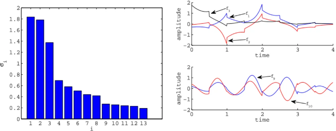
To design the compensation signal, we first compute the singular val-ues and singular vectors. For parameters h = 4 (compensation period) and N = 8, the singular values are computed from Theorem 1 (Fig. 3). The matrix F in (4) is chosen by the solution to the Lyapunov equation
FTF = P : AT
0P + P A0 + I = 0. Figures 4 and 5 depict the normalized
1 2 3 4 5 6 7 8 9 10 11 12 13 0 0.2 0.4 0.6 0.8 1 1.2 1.4 1.6 1.8 2 i σi
Figure 3: Singular values σ1, . . . , σ13.
0 1 2 3 4 −2 −1 0 1 2 time amplitude 0 1 2 3 4 −2 −1 0 1 2 time amplitude f 2 f 3 f 9 f 10 f 1
Figure 4: Normalized singular vectors fi ∈
L2(0, h;R).
vectors corresponding to the small singular values σ9, and σ10tend to exhibit
oscillating behaviors. As mentioned in Remark 2, when the singular vector
f1 corresponding to the largest singular value is applied to the system (26)
(v(t) = f1(t)), the output response z = x is given by σ1·g11(t) = 1.8353·g11(t),
which implies that the system generates a magnified signal of g11(t). Note also that the singular value σi represents the value of the norm of the output gi corresponding to the unit energy input v = fi. When the normalized singular vector f10 corresponding to small singular value σ10is applied to the system, σ10· g101 (t) = 0.2563· g110(t) is generated in the output, which implies that the
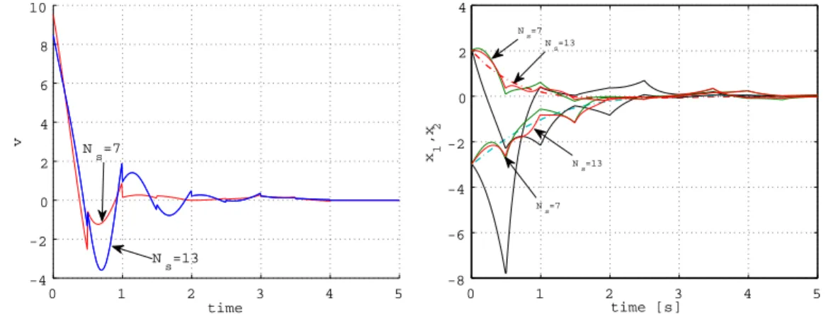
the singular vectors corresponding to the smaller singular values have less of an effect on the input–output relation. Using seven (Ns = 7) singular values
σ1, σ2,· · · , σ7, we design the compensation signal v according to the method
considered in Section 3. Figure 6 shows the compensation signal. The am-plitude around the initial time is larger to improve the large deviation of the original response. Figure 7 shows the state response with compensation. The response approaches that of the average system.
The responses for Ns= 13 are also shown in Figs. 6 and 7. Although the compensation signal for Ns = 13 exhibits similar behavior near the initial time, the amplitude is larger than that of the compensation signal for Ns = 7 after t = 0.5 [s]. Even if we use more singular values, the amplitude would become larger and eliminate only small deviations.
0 1 2 3 4 −1 0 1 time amplitude 0 1 2 3 4 −1 0 1 time amplitude 0 1 2 3 4 −1 0 1 time amplitude 0 1 2 3 4 −1 0 1 time amplitude g 9 g 10 g 1 g 9 g 3 g1 g 2 g2 g 3 g 10
Figure 5: Singular vectors g1
i ∈ L2(0, h;R2)(∥gi∥Z = 1), left:x1, right:x2. 5. Conclusion
In the present paper, we have considered the SVD of an operator repre-senting the input-output relation of a class of linear time-varying systems. The class of the systems describes time-driven switched linear systems. We have derived a computation method for singular values and singular vec-tors of the operator. Based on this SVD, the compensation signal design for switched linear systems with a periodic switching law is discussed. A numerical example was presented in order to demonstrate the fundamental properties of the proposed method.
Although we focus our attention on generating only a continuous-time sig-nal to improve the transient, it would be important to design the switching signal and the continuous-time signal simultaneously. A possible extension of the reseach is incorporating system constraints, which has not been con-sidered in this paper. From practical viewpoint, applying the method to a realistic model is also a topic of future research.
6. Acknowledgement
The first author would like to thank Guisheng Zhai of Shibaura Institute of Technology for providing useful information and comments on examples of switched systems. He also wishes to thank Akira Kojima of Tokyo Metropoli-tan University for his continuous encouragement.
0 1 2 3 4 5 -4 -2 0 2 4 6 8 10 time v N s=7 N s=13
Figure 6: Compensation signal v.
0 1 2 3 4 5 -8 -6 -4 -2 0 2 4 time [s] x1 ,x 2 N s=7 N s=13 N s=13 N s=7
Figure 7: State response with compensation.
Appendix A. Derivation of the adjoint Γ∗ ∈ L(Z, V) in (12)
First, we compute the following inner product:
⟨ˆz, Γv⟩Z =⟨ [ ˆ z0 ˆ z1 ] , [ (Γv)0 (Γv)1 ] ⟩Z = ˆz0T(Γv)0+ ∫ h 0 ˆ z1T(β)(Γv)1(β)dβ. (A.1) The first and second terms in (A.1) are calculated as follows:
(i) first term ˆ z0T(Γv)0 = ˆz0TF N∑−1 s=1 Φ(N,s)(h) ∫ ts ts−1 eAs(ts−τ)B sv(τ )dτ + ˆz0TF ∫ h tN−1 eAN(h−τ)B Nv(τ )dτ = N∑−1 k=1 ∫ tk tk−1 ( BkTeATk(tk−τ)ΦT (N,k)(h)F Tzˆ0)Tv(τ )dτ + ∫ tN tN−1 ( BNTeATN(h−τ)FTzˆ0 )T v(τ )dτ,
(ii) second term ∫ h 0 ˆ z1T(β)(Γv)1(β)dβ = N∑−1 k=1 k ∑ s=1 ∫ tk+1 tk ∫ ts ts−1 ˆ z1T(β)EkΦ(k+1,s)(β)eAs(ts−τ)Bsv(τ )dτ dβ + N ∑ k=1 ∫ tk tk−1 ∫ β tk−1 ˆ z1T(β)EkeAk(β−τ)Bkv(τ )dτ = N∑−1 k=1 ∫ tk tk−1 N∑−1 s=k ∫ ts+1 ts ˆ z1T(β)EkΦ(s+1,k)(β)eAk(tk−τ)Bkdβv(τ )dτ + N ∑ k=1 ∫ tk tk−1 ∫ tk τ ˆ z1T(β)EkeAk(β−τ)Bkdβv(τ )dτ.
For the transformation presented above, we used the reversal of the order of integration and the change in the order of summation. Consequently, by definition (2) of the inner product in V, the adjoint Γ∗ ∈ L(Z, V), which satisfies ⟨ˆz, Γv⟩Z =⟨Γ∗z, vˆ ⟩V, is given by (12).
[1] K. Zhou, J. Doyle, K. Glover, Robust and Optimal Control, Prentice-Hall, 1995.
[2] K. Glover, J. Lam, J. Partington, Rational approximation of a class of infinite-dimensional systems I: Singular values of Hankel operators, Mathematics of Control, Signals, and Systems 3 (1990) 325–344.
[3] Y. Ohta, Hankel singular values and vectors of a class of infinite-dimensional systems: Exact Hamiltonian formulas for control and ap-proximation problems, Mathematics of Control, Signals, and Systems 12 (1999) 361–375.
[4] T. Izumi, A. Kojima, S. Ishijima, Improving transient with compensa-tion law, Proc. of the 15th IFAC World Congress (2002) 181–186. [5] N. Hara, A. Kojima, An off-line design method of compensation law
for constrained linear systems, Int. J. Robust and Nonlinear Control 18 (2008) 51–68.
[6] A. Kojima, M. Morari, LQ control for constrained continuous-time sys-tems, Automatica 40 (2004) 1143–1155.
[7] B. Bamieh, On computing L2-induced norm of finite-horizon systems,
Proc. of the 42nd IEEE Conference on Decision and Control (2003) 1860–1862.
[8] Z. Sun, S. Ge, Switched Linear Systems, Springer, 2005.
[9] I. Masubuchi, G. Zhai, Control of hybrid systems V – analysis and con-trol of switched systems, Systems, Concon-trol and Information 52 (2008) 1860–1862 (in Japanese).
[10] D. Liberzon, Switching in Systems and Control, Birkh¨auser, 2003. [11] X. Xu, P. Antsaklis, Optimal control of switched systems based on
pa-rameterization of the switching instants, IEEE Trans. on Automatic Control 49 (2004) 2–16.
[12] S. Bengea, R. DeCarlo, Optimal control of switched systems based on parameterization of the switching instants, Automatica 41 (2005) 11–27. [13] T. Das, R. Mukherjee, Optimally switched linear systems, Automatica
44 (2008) 1437–1441.
[14] A. V. Savkin, R. J. Evans, Hybrid dynamical systems, Birkh¨auser, 2002. [15] R. W. Brockett, Hybrid models for motion control systems, Essays on Control: Perspectives in the Theory and its Applications (Progress in Systems and Control Theory) (1993) 29–53.