電気通信大学学術機関リポジトリ

(1)

Simulation of a simplified 2D

MHD model of plasma sheet

thinning

Rudolf TRETLER

A dissertation submitted in partial fulfillment of the requirements for the degree of

Doctor of Science

The University of Electro-Communications

Department of Communication Engineering and Informatics

Ch¯

ofu, Tokyo, Japan

(2)

English title: Simulation of a simplified 2D MHD model of plasma sheet thinning

Japanese title: プラズマシート幅の減少に関する 2 次元 MHD

シミュレーション

Advisor: Associate Professor Tomo Tatsuno Secondary advisor: Professor Keisuke Hosokawa

Supervisory committee: Associate Professor Tomo Tatsuno Professor Keisuke Hosokawa Professor Nobito Yamamoto Professor Yoshinobu Nakatani

(3)

c

⃝ 2021 Rudolf Tretler

This work is licensed under the Creative Commons Attribution-ShareAlike 4.0 International License (CC BY-SA 4.0). To view a copy of this license, visit http://creativecommons.org/licenses/by-sa/4.0/.

(4)

(5)

概要オーロラの発生源は、地球磁気圏内の強磁場の磁気ローブに南北から挟まれ、赤道付近で弱磁場の「プラズマシート」と呼ばれる領域にある。プラズマシート内のプラズマ粒子が磁力線に沿って地球方面に流れ、大気の中性粒子と衝突し励起させる。大気の粒子が元の状態に戻るとき、発光してオーロラとして見られる。サブストームという地球磁気圏の乱れによりプラズマ粒子の流れが強くなることがあり、それに伴ってオーロラも増幅され、「オーロラ爆発現象」を起こす。オーロラ爆発現象は磁気圏内のいくつかの物理現象と関連があることがわかっているが、それらの因果関係が未だに解明されていない。この問題を解決する候補の一つである電流擾乱(Current Disruption; CD)モデルによると、プラズマシート内には磁気テイル（太陽と反対側）方面に「希薄波」が伝搬し、地球方面のプラズマ流を引き起こすとされている。プラズマが損失されるにつれて、プラズマシート幅も減少する可能性がある。 ChaoらはCDモデルの簡単な1次元モデルを用いて、希薄波の伝搬と

地球プラズマシートの幅の減少を調べた[J. K. Chao et al., Planet. Space

Sci. 25, 703 (1977)]。その結果が衛星観測等によりCDモデルの正当性を判断するために用いられている。本論文では、Chaoらの1次元モデルを2次元磁気流体(MHD)モデルに拡張し、シミュレーションして解析を行った。まず第1章を序論とし、地球磁気圏の構造、オーロラ爆発現象とそのモデルを紹介した。第2章では、本研究で基礎方程式として用いる理想MHD方程式を保存則形式で導入し、シミュレーション設計に必要な特性分解と連立方程式系の対角化について述べた。第3章では、本論文で用いるシミュレーション手法を解説した。空間差分は不連続性に強いEssentially Non-Oscillatory法、時間差分は3次の Runge-Kutta法を用いた。空間差分の設計には前章の対角化を利用した。第4章では、先行研究であるChaoらが提案した1次元モデルのシミュレーションを行い、結果を確認した。Chaoらは仮想的なピストンを用意し、ピストンを引くと希薄波が発生することを利用してCDモデルを構築した。本研究では2次元への拡張を考え、シート内プラズマの一部に初期速度を与えることで、CDモデルの特徴とされる希薄波をテイル方面に放つこととした。元の1次元モデルでは、希薄波が音速でテイル方面

(6)

に伝搬する。希薄波の通過に伴う圧力の減少はプラズマシート幅の減少を引き起こし、幅の減少も音速で伝達する可能性が示唆されている。第5章では、本題の2次元MHDモデルへの拡張を行い、磁場がない流体としてのシミュレーションと磁場があるプラズマシート構造としてのシミュレーション結果について詳述した。2次元MHDモデルでは、磁場がないプラズマシート領域の北側と南側に接線不連続面で繋がっている強磁場の磁気ローブ領域を追加したことで結果が変わり、希薄波がプラズマシートの圧縮により呑み込まれてほぼ消滅する。しかし、希薄波により引き起こされると考えられていたプラズマシート幅の減少は多少弱まり遅くなるだけで、伝達し続ける。さらに、その伝達速度は1次元モデルとは異なり磁気ローブの磁場の強さに依存していることがわかった。尚、圧力の増加を伴う波列がシート幅の減少を先導する形でシート内に音速でテイル方面に伝搬する。 2次元モデルのシミュレーション結果を物理的に理解するために、波の分解を行った。MHDモデルには7つの波（エントロピー波、正と負の速い磁気音波、正と負の遅い磁気音波、正と負のAlfv´en波）が存在するが、シミュレーション結果をそれらに分解して支配的な成分を特定した。分解して得られた結果は、まず、プラズマシート内での希薄波がほぼ消滅することを確認できた。次に、シート幅の減少の前に伝搬する波列は速い磁気音波として進行していく。また、南北に伝わるシート内の速い磁気音波がシートとローブの境界面に衝突すると、その波の一部がローブに渡り速い磁気音波と遅い磁気音波に分解され、残りが反射してシートに戻ることが観測できた。逆に、ローブ内で励起された遅い磁気音波がシートとの境界面に当たると、その進行速度がゼロになり、境界面で溜まる。速い磁気音波と遅い磁気音波に比べて、エントロピー波の成分が弱く、Alfv´en波が全く励起されていないこともわかった。第6章ではまとめと結論を述べた。モデルを拡張したことで結果が1 次元モデルと比べて大きく変化した。すなわち、1次元モデルで扱えなかったシートとローブの相互作用がプラズマシート幅の減少に大きな影響を与えていることが明らかになった。また、希薄波がほぼ消滅したということは、希薄波の観測の有無は電流擾乱モデルの正当性に繋がらない可能性があることも意味している。さらに、幅の減少とその進行速度が観測データと矛盾しないことが確認された。以上より、現在の観測方法では、CDモデルの正当性を判定することは困難であると考えられる。

(7)

Abstract

There are several competing models trying to explain the physi-cal processes behind auroral breakup, an event where aurora suddenly increases in strength during a magnetospheric substorm. A one dimen-sional (1D) model for thinning of the Earth’s plasma sheet according to the Current Disruption (CD) scenario of auroral breakup was intro-duced by Chao et al. [J. K. Chao et al., Planet. Space Sci. 25, 703 (1977)], and the model’s results form the basis for satellite observations which attempt to determine the CD model’s validity. In this thesis, the 1D model is extended to a simple two dimensional (2D) ideal magne-tohydrodynamic (MHD) configuration and simulated. In both simpli-fied models, an initial disturbance launches a rarefaction wave towards the magnetotail, which is considered a signature component of the CD model.

In this thesis, overview of the problem and the physical background of auroral breakup are described in Chapter 1.

The ideal MHD equations, their properties, and their formulation as a system of conservation laws are introduced in Chapter 2. The diagonalization procedure based on the theory of characteristics, which will be used when constructing the simulation scheme, is also described. The development of the simulation code for the MHD equations in their conservation law formulation is presented in Chapter 3. The spatial integration uses the Essentially Non-Oscillatory (ENO) scheme applied to the diagonalized system of MHD equations, while the time stepping uses the three-stage third-order Runge–Kutta scheme.

Chapter 4 reproduces Chao’s 1D model, where the plasma sheet thinning is modeled in two distinct stages. First, a rarefaction wave propagates tailward at sound velocity, lowering the sheet pressure; sec-ond, the sheet–lobe boundary is assumed to move inwards, reducing the thickness of the plasma sheet. The problem is then reformulated it so it can be extended to 2D.

Chapter 5 is the heart of this thesis; the 1D plasma sheet model is extended to 2D, where the north and south lobe magnetic fields are included in the simulation, simulated under a wide range of parameters,

(8)

and the results analyzed. In the extended model, due to sheet recom-pression, the rarefaction wave is weakened almost to the point of disap-pearance, with a corresponding drastic weakening of the pressure drop in the plasma sheet. However, the thinning continues to propagate, al-beit at a slower velocity than the 1D model suggests; this indicates that the rarefaction wave is not a sole component of plasma sheet thinning. The propagation velocity is also strongly influenced by the strength of the lobe magnetic field, which was outside the scope of the 1D model. Additionally, the thinning front is preceded by a wave train of pulses with slightly increased pressure.

To analyze the simulation results, they were decomposed into their component MHD waves to determine the dominant components. The decomposition confirmed the weakening of the rarefaction wave in the plasma sheet, and showed that the wave train preceding the thinning front consists of fast-mode MHD waves (sound waves). The thinning itself appears to be driven by the slow-mode waves in the magnetic lobes impacting the sheet–lobe boundary, where the slow magnetosonic velocity is sharply reduced, which launches fast-mode waves across the sheet through mode conversion.

Finally, the conclusion is given in Chapter 6, and followed by several appendices. The results of the simulation hint that the presence or ab-sence of the rarefaction wave in the plasma sheet may not be suﬃcient to determine validity of the CD model. Furthermore, a comparison with the observational data shows that the propagation velocity of the thin-ning front and the reduction in sheet thickness are within the plausible range of values. This indicates that current observational methods may not be suﬃcient to prove nor disprove the CD model of auroral breakup.

(9)

Chapter 1 Introduction

Space is big. You just won’t believe how vastly, hugely, mind-bogglingly big it is. I mean, you may think it’s a long way down the road to the chemist’s, but that’s just peanuts to space.

—Douglas Adams, The Hitchhiker’s Guide to the Galaxy

As the late-and-great Douglas Adams so artfully describes, space is vast, and the distances involved are enormous. Unfortunately, this creates some problems when attempting to decipher the physical workings of events tak-ing place oﬀ-planet. The development of space programs and slow but steady reductions in launch costs has allowed for deployment of a great many satel-lites and satellite constellations, whose observational data has been invaluable in determining, among other things, the structure and behavior of Earth’s magnetosphere.

However, due to the aforementioned vastness of space, there are countless mysteries that yet have to be solved. Many of those unsolved problems are connected to events that happen over a wide area, and/or are very infrequent. That makes it diﬃcult to capture enough data for a successful analysis, as the chance that any of the observation satellites might be in the vicinity is fairly low. What we can do, however, is use the limited data to form models, and the (even more meteorical) rise in the computational power to simulate them, checking if and how the model and the observation fit together.

(14)

1.1 General overview

In this thesis, a simplified model of a certain near-Earth event has been sim-ulated and the results analyzed. The event in question occurs in the Earth’s magnetosphere, which is the area around our planet where the Earth’s netic field dominates the Sun’s magnetic field (see section 1.2.1). The mag-netosphere (and interplanetary space in general) is filled with (low-density) plasma, a charged gas where atoms have been dissociated into electrons and ions. When plasma from the magnetosphere is disturbed, some of it may flow down the magnetic field lines into the atmosphere, colliding with the neutral particles, exciting (and often ionizing) them. Photons emitted when the ex-cited particles return to their ground state can be observed as aurora, which is normally expressed as a subdued glow visible in the sky at high latitudes.

A sudden increase in auroral strength, called auroral breakup, can occa-sionally be observed during periods of intense geomagnetic activity [1] (see figure 1.1). While auroral breakup is a highly visible eﬀect, observable from the Earth’s surface, the changes in the Earth’s magnetosphere related to the event are much more diﬃcult to monitor. Due to very large distances and very low matter densities involved, the magnetosphere conditions—even the state of the (relatively) high density area called plasma sheet —cannot be ob-served from the surface of the Earth, and require a direct measurement with a satellite. As mentioned earlier, the distances involved are large (one might even say “astronomical”), and since auroral breakups are rare, there is a very limited amount of observational data. As a consequence, many aspects of the events leading up to and surrounding the auroral breakup have not yet been conclusively determined, and there are many competing models attempting to explain the process [2].

One of the aspects that are not in question is that the auroral breakup oc-curs due to a sudden influx of plasma from the Earth’s plasma sheet into the atmosphere (see section 1.2.4), and the related formation of a near-Earth neu-tral line. However, the ordering of these events is unclear: does the neuneu-tral line form first, pushing plasma towards the Earth and finally into the atmosphere; or does the near-Earth plasma flow into the atmosphere first, thinning the

(15)

(a) The usual, subdued glow of the aurora.

(b) Peak of the auroral breakup.

Figure 1.1: Auroral breakup captured in January 1997 by the visible light camera of the Polar satellite [3]. Public domain images by NASA [4] (the source also includes an animation of the entire event).

plasma sheet and causing the neutral line to form? The former is the assertion of the near-Earth neutral line (NENL) model [5], while the latter is what the current disruption (CD) model [6] states. Currently, most researchers favor the NENL model; however, this thesis focuses on the CD model, simulating the predicted behavior of the plasma sheet and attempting to clarify to what extent the conventional model applies to the observational data. To that end, we focus on what is considered to be the signature aspect of the CD model: a rarefaction wave traveling tailward from the location of the titular current disruption.

In this thesis, we present a simplified two dimensional (2D) magnetohydro-dynamic (MHD) model of the rarefaction wave in the Earth’s plasma sheet. The model is an extension of a one dimensional (1D) model introduced by Chao et al. [7]. Chao’s model employed a piston to generate a rarefaction wave in a 1D gas tube (which represents the inner plasma sheet); a problem with an exact solution which was then extrapolated to the entire plasma sheet (see section 4.1 for details).

While satellite observations of the plasma sheet thinning (for example, the THEMIS mission [8]) have been conducted, and the data analyzed with the intent to ascertain the validity of the CD model, a review of available literature

(16)

has not revealed any simulations of the thinning propagation in the plasma sheet as described by the model. It would appear that the 1D approximation by Chao et al. has been used as a foundation for comparison between CD model’s predictions and observations. However, some problems inherent in the (necessarily rough) approximation can be pointed out. For example, there is no mechanism in the 1D model to account for the eﬀects that the rest of the plasma sheet and the magnetic lobes may have on the behavior of the (magnetically neutral) inner plasma sheet, which may make it deviate from the shape of a 1D rarefaction wave; therefore, the interaction in the 1D piston model is strictly one-directional. Additionally, as will be explained in more detail later on in section 5.8, the propagation velocity of thinning itself is not explicitly stated in the paper; from the way properties of the post-thinning sheet are calculated, it can be concluded that thinning may not even propagate at all.

The 2D MHD model presented in this thesis attempts to improve on the 1D piston model by extending the modeled area to a cross-section of the plasma sheet, including parts of the magnetic lobes. (The physical configuration of the modeled area has been simplified for easier analysis.) By extending the approximation to include the magnetic lobes, we can directly measure the properties of plasma sheet thinning if it were to proceed according to the CD model. Of course, the simulation presented in this thesis is still a simplified version of the CD model, and the results are in no way conclusive. Nevertheless, it does bring us one step closer, and allows us to determine some potential inadequacies of the 1D approximation.

The structure of this thesis is as follows. The physical background, in-cluding a short description of the Earth’s magnetosphere and the two models (NENL and CD), will be presented later in this chapter. The MHD equa-tions, their properties, and their formulation as a conservation law will be introduced in Chapter 2. The simulation scheme and implementation of the self-developed code used to run the simulations in this thesis will be described in Chapter 3. The 1D piston model by Chao et al., as well as an alternative formulation that will be used as a basis of the extension to 2D, will be shown

(17)

in Chapter 4. The aforementioned extension of the plasma sheet model to 2D, as well as the simulation results and their analysis, will be presented in Chapter 5. The conclusion to this thesis is in Chapter 6. Finally, there are several appendices. In Appendix A, the order of the three-step Runge-Kutta method used in the simulation is determined, and in Appendix B the results of some standard numerical tests are presented. Appendix C shows the validity of the simulation domain size through running some of the simulations on a larger domain. Influence of the Kelvin-Helmholtz instability is discussed in Appendix D. Appendix E shows the results of testing a couple of candidate wave decomposition methods (used for analysis of simulation results in sec-tion 5.6) on a linear wave problem. And finally, Appendix F describes some attempts to analytically derive the relationship between the parameters of the plasma sheet and the properties of the thinning, although we ended up here with not much progress.

1.2 Physical background

1.2.1 Earth’s magnetosphere and plasma sheet

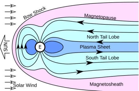
The shape and structure [9] of the Earth’s magnetic field is depicted in fig-ure 1.2, with a more evocative artist’s rendition shown in figfig-ure 1.3. The solar wind, a highly conducting plasma that is emitted by the Sun, carries with itself the Sun’s coronal magnetic field. As the (supersonic) solar wind flows outward, it collides with the magnetic fields of other bodies in the solar system, including Earth, generating a bow shock. As it passes through the bow shock, the solar wind plasma slows down and heats up, creating the magnetosheath (the pink-shaded region in figure 1.2), a region between the bow shock and the Earth’s magnetic field. Since the magnetic field lines cannot interpene-trate, and solar wind plasma, due to the high conductivity, is frozen-in to the Sun’s magnetic field it carries with itself, the solar wind has to deflect around the Earth’s magnetic field. This creates a cavity called magnetosphere (the blue-shaded region in figure 1.2).

(18)

mag-SUN E Plasma Sheet

South Tail Lobe North Tail Lobe Magnetopause Bow Sh

ock

Magnetosheath Solar Wind

Figure 1.2: Rough schematic of the structure of the Earth’s magnetosphere. Supersonic solar wind collides with the terrestrial magnetic field and generates a bow shock. Between the bow shock and the Earth’s magnetic field, which is bounded by magnetopause, is the magnetosheath. The terrestrial magnetic field is deformed by the solar wind pressure, and becomes compressed in front and stretched out in the back (magnetotail). The magnetotail can be further divided into north and south magnetic lobes, with a plasma sheet separating the lobes.

(19)

Figure 1.3: Artist’s rendition of the Earth’s magnetosphere. Image taken from Wikipedia (https://en.wikipedia.org/wiki/File:Magnetosphere_ rendition.jpg); original source NASA (http://sec.gsfc.nasa.gov/ popscise.jpg, no longer available).

netic field generated by the Earth is deformed, with a compressed region in the front, and a stretched-out region in the back, called magnetotail. The magnetotail can further be divided into the north and south magnetic lobes.

The magnetic field lines from the north and south lobes are stretched from the dipole configuration and become almost anti-parallel. As a result, in the center region the magnetic field is weakened, and to keep the entire config-uration balanced, the density and kinetic pressure increase. This region of increased plasma density within a weak magnetic field is called the plasma sheet, or neutral sheet. The typical thickness of the plasma sheet during ge-omagnetically calm periods is 1 to 3RE, where RE denotes the radius of the

Earth, with very high plasma beta values, on the order of β ≈ 100, where plasma beta β = 2µ0p/B2 is the ratio between kinetic pressure p and

mag-netic pressure B2/(2µ0), where B is the magnetic field strength and µ0 is the

magnetic permeability of vacuum.

Flowing dawn to dusk across the plasma sheet is the cross tail current, also known as neutral sheet current. It is a diamagnetic current caused by the gradient in the plasma pressure, and combined with several other currents forms the large-scale magnetospheric current system.

(20)

The shape of the magnetic field lines and the frozen-in property of the plasma dictate that many of the interesting magnetospheric phenomena ob-servable from the Earth’s surface either influence or are influenced by the state of the plasma sheet. In particular, the plasma particles that enter the atmosphere and cause aurora typically originate in the plasma sheet. This is also the reason that the aurora is usually observable only in the far north and south: the magnetic field lines passing through the plasma sheet map to higher latitudes.

1.2.2 Reconnection in the magnetotail

Magnetic reconnection [10] is a physical process where the magnetic field lines rearrange their configuration, releasing the stored magnetic energy. During reconnection, previously unconnected field lines connect to each other, while previously connected field lines separate. The simplest magnetic field config-uration conductive to magnetic reconnection is that of antiparallel magnetic fields, where a thin current sheet separates the fields. Magnetic field lines in such a configuration are easily disturbed (through some instability) and moved closer to each other, dramatically increasing the local gradient of the magnetic field; a small portion of the magnetic flux can diﬀuse through the current sheet, and the magnetic field lines appear to be cut and reconnected in a diﬀerent configuration (see figure 1.4). In the new configuration the mag-netic field lines are under a large amount of tension. As the tension is released, the magnetic field lines move outward from the point of reconnection (in 3D, the reconnection can occur along a line, known as an X-line or a neutral line), carrying plasma in burst flows (jets). (For more details on reconnection see, e.g., Biskamp [10].)

As mentioned in the previous section, the solar wind plasma, carrying with itself the solar magnetic field lines, collides with the Earth’s magnetic field and is deflected around it. The details of the subsequent development have been described by, e.g., Baumjohann & Treumann [9]; here, we will present an abridged version.

(21)

t < 0

t = 0

t > 0

Figure 1.4: The process of magnetic reconnection; diagram based on figure 5.3 from Baumjohann & Treumann [9]. At time t < 0 (left), the two plasmas with antiparallel field lines begin moving towards each other. At time t = 0 (center), the plasmas meet. If there is any diﬀusion across the field lines, the magnetic field may vanish at a point of contact (“neutral point”), cutting the field lines which then get reconnected in a diﬀerent configuration. As the process continues at time t > 0 (right), the plasma flow carries the magnetic field towards the neutral point, where the field lines reconnect, expelling the plasma outwards as the field lines relax into a new configuration.

(22)

it radiates away from the Sun at supersonic and super-Alfv´enic velocity. Due to the Sun’s 27-day rotation, the field lines of the IMF are twisted into a spiral configuration. Where the solar wind impacts the Earth’s magnetosphere, the frozen-in IMF field lines it carries can be either north-facing or south-facing. As the Earth’s magnetic field at the point of contact always faces north, this means that the IMF magnetic field faces south, the field lines at the point of contact will be facing opposite directions, and there will be a merging and reconnection of magnetic field lines on the dayside magnetopause. One side of the merged field lines stays anchored to the Earth, while the other side keeps being carried by the solar wind.

After the dayside reconnection, the merged Earth–IMF magnetic field lines are carried with the solar wind towards the magnetotail. At the far end of the magnetotail, at a distance of approximately 100–200RE, the connected Earth–

IMF field lines reconnect once more, restoring both the closed Earth field line and the open IMF field line. The tailwise transport of the Earth field line stretches out the magnetic field, creating the so-called tail-like configuration (see figure 1.2). As the newly released field line relaxes its magnetic tension, it generates an Earthward plasma flow, and eventually returns to the dayside magnetopause ready for another cycle.

The convection of magnetic field lines from magnetotail back to the dayside does not occur at a uniform rate. As the field lines are released after distant tail reconnection, a part of the magnetic flux stays in the magnetotail, building up and increasing the density of the tail magnetic field lines (i.e., the strength of the magnetic field). The resulting development of the magnetosphere is de-picted in figure 1.5. Once the built up flux passes a certain (variable) threshold, the built up flux suddenly gets released in an explosive reconnection, creating a temporary near-Earth neutral line (NENL), located at 20–30RE. The

near-Earth reconnection has a strong eﬀect on magnetospheric conditions, including the auroral strength, and has been dubbed the magnetospheric substorm. 1

The NENL starts moving tailward, and eventually becomes the new distant 1 _{Occasionally, magnetospheric substorms are precursors to a much stronger disturbance}

called the magnetospheric storm, the details of which are outside of scope of this thesis; see, e.g., Baumjohann & Treumann [9].

(23)

SUN E Plasma Sheet Lobe DNL SUN E DNL NENL SUN E NENL ⇒ DNL Plasmoid Plasmoid Growth Expansion Recovery

Figure 1.5: Tail reconnection and change in the plasma sheet configuration during a magnetospheric substorm; diagram based on figure 5.11 from Baumjo-hann & Treumann [9]. During the growth phase (top), the reconnection at the DNL causes a build up of the magnetic flux inside of the plasma sheet. Af-ter enough flux is transported inwards, the expansion phase (cenAf-ter) starts and the NENL forms, generating a plasmoid between the two neutral lines. The NENL is pushed tailwards in the recovery phase (bottom), expelling the plasmoid into interplanetary space and taking the place as the new DNL.

(24)

neutral line (DNL). After the near-Earth reconnection, the previous DNL is no longer connected to the Earth and is free to be pushed out and released into interplanetary space, carrying with it a portion of magnetospheric plasma.

The signature of the near-Earth reconnection and the formation of the NENL has been observed by the satellites. Figure 1.6 shows the observational data the Geotail satellite took as it was passing close to the location where a neutral line formed, presented by Asano et al. [11]. Between times of 11:55 and 12:05, the satellite observed large changes in the plasma sheet properties, consistent with the behavior during reconnection. The density fell, accompa-nied by a rise in ion and electron temperatures. There was also a large increase in plasma flow velocity, with a large diﬀerence between ion and electron com-ponents. The velocity moments were used to determine the structure of the current sheet (region of strong current in the inner plasma sheet) around the NENL, with the analysis showing that the thickness of the current sheet is re-duced to around 500 km, compared to the local ion inertial length of∼ 720 km. A Hall current system [9], which typically forms around a neutral line, is also present.

Note that in this thesis, the magnetotail reconnection itself is not modeled, as it is not possible for it to occur under the ideal MHD model we will be using (see Chapter 2).

1.2.3 Cross tail current disruption

Around the time of the formation of the NENL at 20–30RE, the near-Earth

cross tail current also experiences a strong disturbance [12] at a distance of around 10RE down the magnetotail. The cross tail current, which is aligned

with the equatorial plane, forms a so-called substorm current wedge [9]; it is diverted on the morning side to flow along the magnetic field lines into the ionosphere, returning back to the plasma sheet on the evening side.

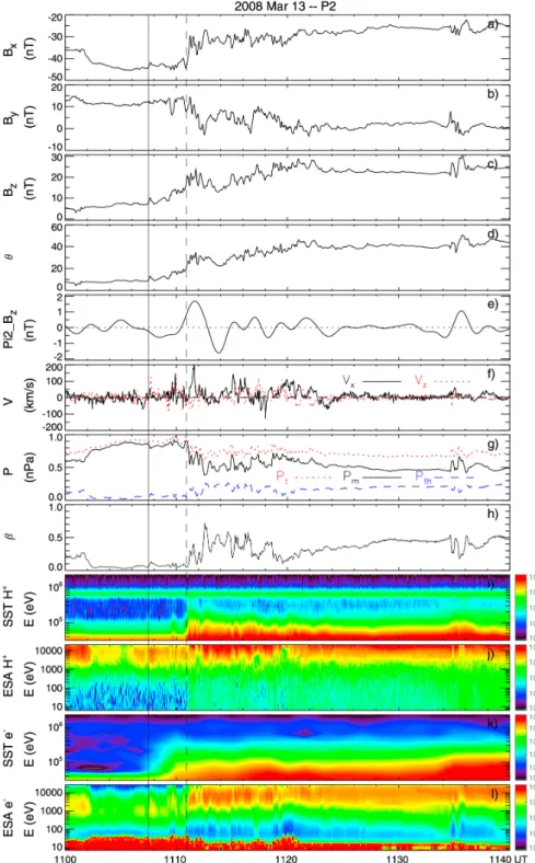
Satellite observations of current disruption are numerous; see, for example, Takahashi et al. [13], Lui et al. [14], Tang et al. [15]. Figure 1.7 shows a current disruption event in March 2008 as observed by the satellite P2 of the THEMIS constellation, reproduced from figure 7 in the paper by Tang et al. [15]. Plotted

(25)

Figure 1.6: Observational data of an NENL event, taken by the Geotail satel-lite. Plotted values are the total magnetic field BT and it’s components Bx,

By, and Bz (where x points sunward, and z points north); numerical density

N , temperature T , and the three velocity components vx, vy, and vz of the

plasma; the cross tail current density jy; and the total pressure P (black) and

thermal pressure P p (blue). Where available, separate values for ions (red) and electrons (blue) are shown. Figure taken from Asano et al. [11]; see the referenced paper for detailed discussion.

(26)

values are the magnetic field components Bx, By, and Bz (where x points

sunward, and z points north); the elevation of the magnetic field θ (where 0◦ is tail-like, and 90◦ is dipolar); pulses in Bz in the period range of 40–

150 s; ion velocity components vx (black solid line) and vz (red dotted line);

magnetic pressure Pm (black solid line), kinetic (thermal) pressure Pth (blue

dashed line), and total pressure Pt (red dotted line); plasma beta β; energy

spectra of ions and electrons, obtained by two separate instruments. The vertical solid line denotes the onset of flux pileup, while the vertical dashed line denotes the onset of current disruption. As the cross-tail current is not observed directly, the disruption event has to be inferred, mainly from the behavior of the magnetic field. Here, a sharp decrease in |Bx| around 11:11

marks the start of the current disruption near the satellite’s location. This sudden drop in |Bx| is accompanied by an equally sudden increase in average

energy of ions and electrons, plasma kinetic pressure, and plasma beta, as well as plasma density and temperature (not shown). At the same time, there is a drop in magnetic pressure and total pressure. These changes are taken to be a clear indicator of current disruption.

Near-Earth magnetotail reconnection and current disruption are connected, though exact causal relationship is so far unknown, and the mechanism behind the magnetotail current disruption has not yet been conclusively determined. One possible explanation [9] is that the magnetic flux carried by the Earthward plasma flow generated by the formation of the NENL (see the following section) piles up in the inner magnetosphere, where the magnetic field lines change from a stretched-out, tail-like configuration, into a dipole configuration. The flux pileup causes the depolarization of the tail magnetic filed, which also reduces the cross-tail current in that region; the excess current trying to move through is forced to divert into the ionosphere as field aligned currents.

Some of the other candidate models for current disruption, which do not require the NENL to form beforehand, are the magnetosphere–ionosphere cou-pling (MIC) model and the Ballooning Instability (BI) model [12]. In the MIC model [16], the dayside reconnection launches an Alfv´en wave into the night-side plasma sheet, where the current in the wave interacts with the cross tail

(27)

Figure 1.7: Observational data of a current disruption event, taken by one of the THEMIS satellites. Plotted values are described in the main text. Figure taken from Tang et al. [15]; see the referenced paper for detailed discussion.

(28)

current, reducing it. This interaction bounces the Alfv´en wave into ionosphere, which bounces it right back, further disturbing the current, and so on; the pos-itive feedback creates an instability and diverts the current into the ionosphere. According to the BI model [17], the transition in magnetic field configura-tion from tail-like to dipolar is analogous to a heavy fluid resting on top of a light fluid; therefore, the configuration is vulnerable to the development of a Rayleigh–Taylor instability. As the ballooning modes grow due to the insta-bility, they cause growth of polarization electric fields, resulting in a charge buildup in the region. Neutralizing the excess charge causes the field aligned currents to form.

1.2.4 Auroral breakup

During magnetic substorms, periods of intense geomagnetic activity, a sudden and dramatic increase in auroral strength can sometimes be observed [1]. This event is called auroral breakup, or auroral explosion, and the mechanism behind it is not yet entirely understood. There are certain sub-events that are known to occur during or before auroral breakup [18] (see figure 1.8), namely,

(a) magnetotail reconnection, (b) cross tail current reduction, and

(c) auroral breakup itself.

However, the exact order of these events, and therefore their precise causal relationship, has not yet been conclusively determined. The two primary com-peting models that try to explain these events and how they relate to each other are the Near-Earth Neutral Line (NENL) model [5] and the Current Disruption (CD) model [6].

Near-Earth Neutral Line model

In the Near-Earth Neutral Line model, a disturbance in the magnetotail, caused by the solar wind, induces a reconnection of the stretched-out, an-tiparallel magnetic field lines (sub-event (a)). The magnetic reconnection is

(29)

SUN E Plasma Sheet

South Lobe North Lobe

Auroral Breakup

Cross Tail Current Reduction

Magnetotail Reconnection

Figure 1.8: Approximate relative locations of the sub-events (marked in blue) related to auroral breakup. The cross tail current reduction occurs at a dis-tance of ∼ 6–10RE tailward from the Earth [2] The tail reconnection takes

place at a distance of ∼ 20–30RE. The auroral breakup itself occurs in the

upper regions of the atmosphere.

a high-energy event which creates jets of plasma that flow Earthward and tailward. The passage of the Earthward jet causes a decrease in the cross tail current (sub-event (b)), and finally the jet enters the high-latitude atmosphere, where it causes the auroral breakup (sub-event (c)).

The NENL model has been simulated frequently; for example, a cursory search of the literature has revealed papers from 1981 by Lyon et al. [19], with a 2D global MHD simulation, to 1993 by Walker et al. [20] and 2010 by Tanaka et al. [21], both with a 3D global MHD simulation.

Current Disruption model

In the Current Disruption model, first the cross tail current is reduced (sub-event (b)) through, as the name indicates, a current disruption instability. As a result, the balance of the near-Earth magnetotail plasma is broken, and the resulting plasma flow enters the high-latitude atmosphere and causes the auroral breakup (sub-event (c)).

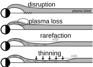
On the opposite side, the plasma loss in the magnetotail induces a rar-efaction wave that starts propagating tailward through the plasma sheet (fig-ure 1.9). The passage of the rarefaction wave causes the plasma sheet press(fig-ure

(30)

disruption

plasma loss

rarefaction

thinning

Figure 1.9: The process of plasma sheet thinning as described by the CD model. Image adapted from Chao et al. [7].

to drop, the sheet–lobe boundary moves inward, and plasma sheet thickness is reduced. As the antiparallel magnetic field lines move closer to each other, they eventually trigger the magnetotail reconnection (sub-event (a)).

It may be worth pointing out that while there is a strict ordering to the sub-events in the NENL model, in the CD model the auroral breakup and magnetotail reconnection are not parts of the same causal chain. While both sub-events are caused by the same precursor, their relative ordering is not determinable.

A possible mechanism by which the disruption of the cross-tail current may generate an Earthward flow of plasma is presented by Shiokawa et al. [22], based on the analysis of the observational data from the Geotail satellite. The mechanism is summarized in figure 7 of Shiokawa et al. [22], reproduced here (with minor edits) in figure 1.10. The steps are as follows. (a) During calm periods, the extended, tail-like configuration of the magnetic field lines is sup-ported by the plasma pressure gradient −∇p (pushing the plasma tailward) acting against the Lorentz force j× B (pushing the plasma Earthward). (b) The growth phase of the substorm strengthens the cross-tail current, further enhancing the tail-like nature of the magnetic field in the near-Earth region. (c) However, the intense eﬀects of a substorm cause an instability, possibly

(31)

Figure 1.10: A possible mechanism by which an Earthward flow of plasma can be caused by the disruption of near-Earth cross-tail current; image taken from Shiokawa [22]. The steps (a) to (f) are explained in the main text.

(32)

by one of the mechanisms introduced above; (d) a localized disruption reduces the cross-tail current, strengthening the magnetic field on the Earth side of the disruption, and weakening it on the tail side. (e) The changes in the Lorentz force break the balance, generating a plasma flow inwards and outwards, away from the disruption. (f) Finally, the plasma loss due to the Earthward flow reduces the plasma pressure gradient, which causes the entire plasma to flow Earthward, initiating the auroral breakup in the upper atmosphere (and, pre-sumably, the thinning of the plasma sheet in the magnetotail).

Note that, unlike the more popular NENL model, an extended search of literature has not surfaced any direct simulations of the CD model. The only relevant paper we were able to find is a 1977 paper by Chao et al. [7], which uses an extremely simplified 1D model of the plasma sheet.

Observations

The primary diﬃculty with determining which of the candidate models (if any) is the correct one is the sheer scale of the problem. While there is observational data for specific sub-events: the current disruption [12, 14, 22], the plasma flow, the change in direction of the magnetic field, and what appears to be the formation of the near-Earth neutral line [11]; the distances involved are such that the most we can obtain is point data at the location of a satellite that is by chance passing by. However, both of the above models involve a large-scale disturbance and reconfiguration of the plasma sheet and the surrounding magnetic field.

As an example, detecting a thinning of the plasma sheet would require finding out the location and time evolution of the sheet–lobe boundary over a distance of 10–20RE during a period of ∼ 10 minutes. However, with a point

observation from a moving platform, we are only able to detect the magnetic field strength and particle density at a certain location in the magnetotail. If there is a sudden drop in density and the magnetic field, it may signify that the thinning front moved over the satellite, albeit whether the propagation is Earthward or tailward is unknowable without additional points of observation. On the other hand, as the sheet is not stationary, that particular observation

(33)

may also signify that the entire sheet moved southwards or northwards, without any thinning at all. We can conclude that the direct observation of thinning would require wide-area detection instruments far beyond the current tech-nology level and/or orders of magnitude larger budgets for satellite launches, neither of which are presently available. The models of plasma sheet thinning have to build on the fragmentary observations currently obtainable, filling in the missing pieces with theoretical analysis; the NENL model and the CD model introduced above are two examples of such analysis.

Nevertheless, the science slowly marches on. About a decade ago, the THEMIS mission [8] tried to determine which of these two models is the one explaining the auroral substorms and the related auroral breakup. Satellite part of the THEMIS mission is composed of five identical satellite probes distributed and coordinated in the tail of the magnetosphere, which enables us to observe the disturbances in the magnetotail leading to the auroral substorm. To support the satellite observations in space, a number of all-sky cameras were deployed in North America to observe the signature of auroral breakup at the magnetic footprints of the satellites [23]. By using the data obtained by the THEMIS mission, Angelopoulos et al. [24] demonstrated an event in which reconnection took place at−20RE a few minutes earlier than the signature of

current disruption at∼ −10RE. This observation supports the NENL model,

that is, that auroral substorms are initiated by reconnection in the magnetotail. Later, however, Lui [25] claimed that multi-satellite observations during the same interval can be interpreted based on the CD paradigm. Thus, it is still controversial which of these two models better explains the development of the magnetotail disturbances before auroral breakups, and can be regarded as the dominant triggering mechanism of substorms.

(34)

Chapter 2 Ideal MHD model

To describe plasma in a precise, physically correct way would require solving a kinetic equation for the particle distribution function over the entire phase space (three spatial and three velocity dimensions). However, this approach is extremely computationally expensive, and the results are more detailed than is necessary in many cases. In physical domains such as the plasma sheet, we are more often interested in large-scale features of the plasma, including its velocity, density, and pressure.

2.1 Ideal MHD equations

In the magnetohydrodynamic (MHD) model, plasma is treated as an ionized fluid. The MHD equations are obtained by integrating the Vlasov equation over the velocity space for each component particle species (multi-fluid theory) and combining them with the Maxwell’s equations of electrodynamics [9]. To obtain single-fluid MHD equations, there is a further assumption that there are only two relevant species, electrons and protons, with equal charge densities (quasi-neutrality), and the equations can be expressed for the center of mass of the two fluids [9, 26]. By neglecting the viscosity, thermal conductivity, and resistivity [27, 28], and assuming slow variations (neglecting the displacement

(35)

current), we can obtain the ideal MHD equations, ∂ρ ∂t +∇ · (ρu) = 0, (2.1) ∂u ∂t + u· ∇u + 1 ρ∇p − 1 µ0ρ (∇ × B) × B = 0, (2.2) ∂p ∂t + u· ∇p + γp∇ · u = 0, (2.3) ∂B ∂t − ∇ × (u × B) = 0, (2.4) ∇ · B = 0, (2.5)

where ρ is the density, p is the kinetic pressure, u = (u, v, w) is the velocity vector, B = (Bx, By, Bz) is the magnetic field vector, γ is the ratio of specific

heats, and µ0 is the magnetic permeability of vacuum.

For the CD model of the auroral breakup in the Earth’s plasma sheet, we can describe three distinct phases of development. First is the current disruption phase, which is possibly dominated by the small-scale kinetic eﬀects outside the scope of the MHD theory [12]. Second is the rarefaction wave phase, where the spatial scale is long, and temporal variations are slow; the ideal MHD approximation is justified for this phase. Finally, the third phase is the reconnection phase; since under the ideal MHD theory the magnetic filed lines can never cross each other, that theory is, again, inapplicable. Therefore, the ideal MHD model can be safely used only for the middle phase: after the current disruption is over, and until the reconnection begins.

2.2 Conservation laws

A conservation law states that some physical quantity does not change with time; for example, a conservation of mass or conservation of momentum. These quantities are often called conserved variables (e.g., momentum, energy), in contrast to primitive or physical variables (e.g., velocity, pressure). It is often beneficial to form a system of equations in terms of conserved variables, as it unlocks a wide range of numerical methods and analysis approaches [29].

(36)

are ∂U ∂t + ∂F ∂x + ∂G ∂y + ∂H ∂z = 0, (2.6)

with state vector U = U(x, y, z, t) and fluxes F = F(U), G = G(U), H =

H(U) in x, y, z directions.

In 1D systems, we assume that physical properties vary only in the x direc-tion, while being homogeneous in y and z directions. This significantly reduces the complexity of the problem and allows us to considerably simplify the PDEs describing it. Conservation laws in 1D reduce to

∂U ∂t +

∂F

∂x = 0 (2.7)

with U = U(x, t) and a single flux F = F(U) in the x direction. Using the Jacobian matrix A(U) = ∂F ∂U =     ∂F1 ∂U1 · · · ∂F1 ∂Uk .. . . .. ... ∂Fk ∂U1 · · · ∂Fk ∂Uk     , (2.8)

where k denotes the size of the state vector U, we can rewrite equation (2.7) as

∂U

∂t + A(U) ∂U

∂x = 0. (2.9)

If all of the eigenvalues of the Jacobian matrix A(U) are real and it has a complete set of right eigenvectors, then we say that the system (2.9) is hyper-bolic [29].

2.3 Ideal MHD equations as a conservation

law

Formulation in 3D

We use the ideal MHD equations in their formulation as a system of conser-vation laws [30]. A system of conserconser-vation laws in 3D can be represented as

(37)

∂U ∂t + ∂ ∂xF(U) + ∂ ∂yG(U) + ∂ ∂zH(U) = 0, (2.10) where U is a vector of conserved variables and F(U), G(U), and H(U) are respectively fluxes in x, y, and z directions. For the ideal MHD system, the conserved variables are

U = (ρ, ρu, ρv, ρw, Bx, By, Bz, e)⊺, (2.11)

where ρ is the density, u = (u, v, w) is the velocity vector, B = (Bx, By, Bz)

is the magnetic field vector, and e is the total energy density. Manipulating the equations (2.1)–(2.5) into the conservation form (2.10), the fluxes in (2.10) become F(U) =                  ρu ρuu− _µ1 0BxBx+ ptotal ρvu− _µ1 0BxBy ρwu− _µ1 0BxBz 0 Byu− Bxv Bzu− Bxw u(e + ptotal)− _µ1 0Bx(u· B)                  , (2.12) G(U) =                  ρv ρuv−_µ1 0ByBx ρvv− _µ1 0ByBy + ptotal ρwv−_µ1 0ByBz Bxv− Byu 0 Bzv− Byw v(e + ptotal)−_µ1 0By(u· B)                  , (2.13)

(38)

H(U) =                  ρw ρuw− _µ1 0BzBx ρvw− _µ1 0BzBy ρww− _µ1 0BzBz + ptotal Bxw− Bzu Byw− Bzv 0 v(e + ptotal)− _µ1₀Bz(u· B)                  , (2.14)

where µ0 = 4π × 10−7 H m−1 is the magnetic permeability of vacuum, and

total pressure ptotal is ptotal = p +

1 2µ0

B· B (2.15)

with pressure p defined as p = (γ− 1) ( e− 1 2ρu· u − 1 2µ0 B· B ) , (2.16)

where γ is the ratio of specific heats.

The formulation of conservation law in 2D is ∂U ∂t + ∂ ∂xF(U) + ∂ ∂yG(U) = 0, (2.17)

where the fluxes F(U) and G(U) are the same as in the formulation in 3D.

The formulation of conservation law in 1D is ∂U

∂t + ∂

∂xF(U) = 0, (2.18)

and the divergence condition (2.5) dictates that Bx must be constant in space.

The component equation for Bx becomes ∂Bx/∂t = 0, and the system can be

reduced to seven variables,

(39)

with a seven-component flux F′(U′) =               ρu ρuu−_µ1 0BxBx+ ptotal ρvu− _µ1 0BxBy ρwu−_µ1 0BxBz Byu− Bxv Bzu− Bxw u(e + ptotal)−_µ1₀Bx(u· B)               (2.20) in the x direction.

2.4 Normalization

To further simplify the formulation (and ease the implementation), we normal-ize the equations by scaling all quantities φ by their respective normalization parameters, φ = ˆφ ¯φ, where ¯φ are the normalized quantities, and the constants

ˆ

φ are the normalization parameters. Specifically, the normalization parameters for the ideal MHD equations are

ρ = ˆρ ¯ρ, u = ˆu¯u, Bx = ˆBxB¯x, x = ˆx¯x,

e = ˆe¯e, v = ˆv¯v, By = ˆByB¯y, y = ˆy ¯y,

p = ˆp¯p, w = ˆw ¯w, Bz = ˆBzB¯z, z = ˆz ¯z,

t = ˆt¯t.

(2.21)

Substituting (2.21) into MHD equations, we obtain the constraints that the parameters must satisfy. First set of constraints,

ˆ x = ˆy = ˆz, (2.22) ˆ u = ˆv = ˆw, (2.23) ˆ Bx = ˆBy = ˆBz = √ µ0p,ˆ (2.24) ˆ p = ˆe, (2.25)

defines parameter groups, while the second set, ˆ

x = ˆuˆt, (2.26)

ˆ

(40)

defines relationships between them. The parameter groups are distance, ve-locity, energy, density, and time. Here, energy is strongly coupled with mag-netic field (2.24) and pressure (2.25). We can choose three of the parameters from (2.26)–(2.27) as free parameters, with the other two as dependents.

We define ¯U as a vector of normalized conserved variables, and ¯F( ¯U) and

¯

G( ¯U) as normalized fluxes in ¯x and ¯y normalized directions. With this con-vention, normalized conserved variables in 2D become

¯

U =(ρ, ¯¯ ρ¯u, ¯ρ¯v, ¯ρ ¯w, ¯Bx, ¯By, ¯Bz, ¯e

)_⊺

. (2.28)

Normalized fluxes become

¯ F( ¯U) =                  ¯ ρ¯u ¯ ρ¯u¯u− ¯BxB¯x+ ¯ptotal ¯ ρ¯v ¯u− ¯BxB¯y ¯ ρ ¯w¯u− ¯BxB¯z 0 ¯ Byu¯− ¯Bxv¯ ¯ Bzu¯− ¯Bxw¯ ¯ u(¯e + ¯ptotal)− ¯Bx(¯u· ¯B)                  , (2.29) ¯ G( ¯U) =                  ¯ ρ¯v ¯ ρ¯u¯v− ¯ByB¯x ¯ ρ¯v¯v − ¯ByB¯y+ ¯ptotal ¯ ρ ¯w¯v− ¯ByB¯z ¯ Bxv¯− ¯Byu¯ 0 ¯ Bz¯v− ¯Byw¯ ¯ v(¯e + ¯ptotal)− ¯By(¯u· ¯B)                  , (2.30)

(41)

¯ H( ¯U) =                  ¯ ρ ¯w ¯ ρ¯u ¯w− ¯BzB¯x ¯ ρ¯v ¯w− ¯BzB¯y ¯ ρ ¯w ¯w− ¯BzB¯z+ ¯ptotal ¯ Bxw¯− ¯Bzu¯ ¯ Byw¯− ¯Bz¯v 0 ¯ v(¯e + ¯ptotal)− ¯Bz(¯u· ¯B)                  , (2.31)

where ¯ptotal is the total pressure

¯

ptotal = ¯p +

1

2B¯ · ¯B (2.32)

with pressure ¯p defined as

¯ p = (γ − 1) ( ¯ e−1 2ρ¯¯u· ¯u − 1 2 ¯ B· ¯B ) . (2.33)

In 1D, the vectors of conserved variables ¯U and flux ¯F can be formed by

dropping the ¯Bx component. For simplicity, we will henceforth drop the bars

and refer exclusively to the normalized version of the MHD equations (2.28)– (2.33).

2.5 Galilean invariance

Let the inertial frame K′ be moving with constant relative velocity V,|V| ≪ c, with respect to the reference frame K. With no loss of generality, we can assume that V = (V, 0, 0) (figure 2.1). Then, the Galilean transformations for

(42)

x

y

x'

y'

K

K'

V

Figure 2.1: Coordinate systems of the reference frame K (solid axes) and inertial frame K′ (dotted axes). The inertial frame moves with a constant velocity V = (V, 0, 0) with respect to the reference frame.

parameters of frame K′ and an MHD plasma in that frame are [31] t′ = t, (x′, y′, z′) = (x− V t, y, z), (u′, v′, w′) = (u− V, y, z), ρ′ = ρ, (2.34) p′ = p, B′ = B. Expressing t′ = t′(x, y, z, t), x′ = x′(x, y, z, t), y′ = y′(x, y, z, t), and z′ = z′(x, y, z, t), we can obtain the partial derivatives of all pairs of coordinates,

∂t′/∂t = 1, ∂t′/∂x = 0, ∂t′/∂y = 0, ∂t′/∂z = 0, ∂x′/∂t =−V, ∂x′/∂x = 1, ∂x′/∂y = 0, ∂x′/∂z = 0, ∂y′/∂t = 0, ∂y′/∂x = 0, ∂y′/∂y = 1, ∂y′/∂z = 0, ∂z′/∂t = 0, ∂z′/∂x = 0, ∂z′/∂y = 0, ∂z′/∂z = 1.

(2.35)

Substituting the above into the partial derivatives of a plasma property φ′ in the inertial frame K′ with respect to the reference frame K, through the chain rule we obtain ∂φ′ ∂t = ∂φ′ ∂t′ ∂t′ ∂t + ∂φ′ ∂x′ ∂x′ ∂t + ∂φ′ ∂y′ ∂y′ ∂t + ∂φ′ ∂z′ ∂z′ ∂t = ∂φ ′ ∂t′ − V ∂φ′ ∂x′, (2.36)

(43)

and with the equivalent calculation ∂φ′ ∂x = ∂φ′ ∂x′, ∂φ′ ∂y = ∂φ′ ∂y′, ∂φ′ ∂z = ∂φ′ ∂z′. (2.37)

Taking the density component of the MHD system expressed in the refer-ence frame K, ∂ρ ∂t + ∂ ∂x(ρu) + ∂ ∂y(ρv) + ∂ ∂z(ρw) = 0, (2.38)

and substituting the Galilean transformations in (2.34), we obtain ∂ρ′ ∂t + ∂ ∂x(ρ ′_u′_{+ ρ}′_{V ) +} ∂ ∂y(ρ ′_v′_{) +} ∂ ∂z(ρ ′_w′_{) = 0.} _(2.39)

Applying the chain rules from (2.36) and (2.37), the equation transforms into ∂ρ′ ∂t′ − V ∂ρ′ ∂x′ + ∂ ∂x′(ρ ′_u′_{) + V} ∂ρ′ ∂x′ + ∂ ∂y′(ρ ′_v′_{) +} ∂ ∂z′(ρ ′_w′_{) = 0,} _(2.40)

that can be simplified into ∂ρ′ ∂t′ + ∂ ∂x′(ρ ′_u′_{) +} ∂ ∂y′(ρ ′_v′_{) +} ∂ ∂z′(ρ ′_w′_{) = 0,} _(2.41)

which is the density component of the MHD system in the inertial frame K′. Comparing equation (2.41) with the density component in the reference frame K from (2.38), it is clear that the density equation is Galilei invariant.

Obtaining the transforms ptotal = p′total and e = e′ + 1 2ρ′V

2 _{+ ρ}′_u′_{V , and}

performing equivalent transformations on the other seven MHD equations, after some simple manipulations it is easily confirmed that all eight MHD equations are Galilei invariant.

2.6 System of equations

A single-component conservation law, where the vector of conserved variables

U consists of a single element, is relatively easy to discretize (see section 3.1.3).

Properly extending the aforementioned discretization method to a system of equations (see section 3.1.4) requires the use of the theory of characteristics.

(44)

2.6.1 Characteristics

Characteristics or characteristic curves of a partial diﬀerential equation (PDE) of a scalar variable u(x, t) are curves x = x(t) in the t-x plane along which the PDE becomes an ordinary diﬀerential equation (ODE) [29]. For the 1D advection equation, which is a PDE of the form

∂u ∂t + a

∂u

∂x = 0, (2.42)

and taking x = x(t), the rate of change du/dt along the curve x = x(t) is du dt = ∂u ∂t + dx dt ∂u ∂x. (2.43) If we set dx dt = a, (2.44)

where a is called the characteristic speed, then from the equation (2.43) the rate of change du/dt along the curve x = x(t) becomes zero; in other words, u is constant along the said curve.

2.6.2 Diagonalization

Another concept that will be used in section 3.1.4 to discretize a system of equations is the diagonalization of said system.

We define the matrices Λ and R as

Λ =     λ1 0 . .. 0 λk     and R = (R1, . . . , Rk), (2.45)

where λj (j = 1, . . . , k) are the eigenvalues, R is a square matrix of order k

whose column vectors of k components Rj are the right eigenvectors of the

system’s Jacobian A, where A is defined by equation (2.8). For a system with one variable the Jacobian A degenerates into the characteristic speed a (see 2.6.1). For a hyperbolic system—which we assume our conservation law to be—all of the right eigenvectors are linearly independent, and consequently the

(45)

matrix R is non-singular. Inverting the matrix R, we get the matrix L = R−1, L =     L1 .. . Lk     , (2.46)

where L is a square matrix of order k whose the row vectors of k components Lj are the left eigenvectors of the Jacobian matrix A. The matrix L is the

inverse of matrix R, L = R−1.

Multiplying the Jacobian A from left and right with L and R, respectively, we obtain

LAR = Λ. (2.47)

If the matrices A, Λ, R and L are constant, we can use the identity (2.47) to rewrite (2.9) to obtain L∂U ∂t + (LAR)L ∂U ∂x = 0 ∂W ∂t + Λ ∂W ∂x = 0 (2.48)

where W = LU is a state vector of characteristic variables. It is immediately obvious that (2.48) is a set of k independent advection equations

∂Wj

∂t + λj ∂Wj

∂x = 0, (j = 1, . . . , k) (2.49)

with eigenvalues λj as wave speeds (characteristic speeds).

For the 1D normalized ideal MHD equations, with flux (2.20), the wave speeds λj are, in non-decreasing order (and independent of the value of β),

λ1 = u− cfm, λ2 = u− cA, λ3 = u− csm, λ4 = u, (2.50) λ5 = u + csm, λ6 = u + cA, λ7 = u + cfm,

where cA is the Alfv´en speed

cA=

√ B2

x

(46)

and cfm and csm are, respectively, the fast and slow magnetosonic speeds, cfm = v u u u t1 2  c2 s + B· B ρ + √( c2 s + B· B ρ )2 − 4c2 sc2A   (2.52) csm= v u u u t1 2  c2 s + B· B ρ − √( c2 s + B· B ρ )2 − 4c2 sc2A  , (2.53)

with sound speed cs defined as

cs=

√ γp

ρ . (2.54)

Complete sets of right and left eigenvectors of the 1D MHD system are given, respectively, by Brio & Wu [32] and Ryu & Jones [27]. The eigenvectors have been renormalized to remove the singularities.

Note that the eigenvalues of the MHD equations’ Jacobian depend on the conserved variables U; the same is true for the matrices A, R and L. Thus, it would appear that the MHD system cannot be decomposed into independent advection equations (2.49). This problem will be addressed in section 3.1.4.

(47)

Chapter 3 Simulation code

The simulations in this thesis have been run on a self-developed C++ simu-lation code, and the results analyzed with an ad-hoc hodge-podge of gnuplot scripts, Perl scripts, and spreadsheets.

3.1 Simulation scheme

The simulation method is constructed in two steps, using the so-called method of lines. A 1D PDE for a conserved physical quantity u(x, t) and flux f (u(x, t)) is

∂u ∂t +

∂f (u)

∂x = 0. (3.1)

Leaving the time variable in the MHD equations continuous, we discretize only the spatial derivative,

L(u)≈ −∂f (u(x, t))

∂x , (3.2)

where L is an operator denoting a discretized approximation where the time variable is left continuous. The partially discretized PDE can then be rewritten as

∂u

∂t = L(u), (3.3)

and the time derivative can now also be discretized independently with a suit-able time stepping scheme.

(48)

3.1.1 Problem properties

The traditional computational schemes (e.g., central finite diﬀerence), when applied to conservation laws, reconstruct the numerical flux from a stencil fixed in both space and time. One of the problems with a fixed stencil emerges when there exists a shock (discontinuity) in the physical variables. In problems that include shocks, fixed stencils produce solutions with pronounced non-physical oscillations, known as Gibbs phenomena.

There are several ways of dealing with Gibbs phenomena. Among those, the Essentially Non-Oscillatory (ENO) schemes for hyperbolic conservation laws introduced by Harten et al. [33] are among the most robust, with reason-ably sharp shock resolutions, on the order of several computational cells, and no discernible accuracy penalty. Conversely, the relative diﬃculty of imple-mentation and computational cost of the ENO schemes have to be considered before deciding on their use. Since the goal of this research is to simulate the rarefaction wave in the Earth’s plasma sheet, the positive sides of ENO scheme will be necessary, thus the penalties are acceptable.

3.1.2 TVD schemes

Total Variation Diminishing (TVD)—also sometimes known as Total Variation Non-Increasing (TVNI)—schemes [34, 35] are a class of numerical schemes where the total variation T V of a discretized variable u, defined as

T V (u) =∑

i

|ui+1− ui|, (3.4)

satisfies the condition

T V (u(n+1))≤ T V (u(n)) (3.5) where T V (u(n)_{) is the total variation at time step n.}

TVD schemes are convergent and monotonicity preserving. Furthermore, as the total variation is bounded, oscillations such as the Gibbs phenomena are unable to develop. The downside is that the accuracy is limited; linear TVD schemes have first-order accuracy. However, nonlinear TVD schemes such as ENO can have second-order or higher accuracy.

電気通信大学学術機関リポジトリ

Simulation of a simplified 2D

MHD model of plasma sheet

thinning

Rudolf TRETLER

The University of Electro-Communications

Department of Communication Engineering and Informatics

Ch¯

ofu, Tokyo, Japan

Contents

Chapter 1

Introduction

1.1

General overview

1.2

Physical background

1.2.1

Earth’s magnetosphere and plasma sheet

1.2.2

Reconnection in the magnetotail

t < 0

t = 0

t > 0

1.2.3

Cross tail current disruption

1.2.4

Auroral breakup

disruption

plasma loss

rarefaction

thinning

Chapter 2

Ideal MHD model

2.1

Ideal MHD equations

2.2

Conservation laws

2.3

Ideal MHD equations as a conservation

law

2.4

Normalization

2.5

Galilean invariance

x

y

x'

y'

K

K'

V

2.6

System of equations

2.6.1

Characteristics

2.6.2

Diagonalization

Chapter 3

Simulation code

3.1

Simulation scheme

3.1.1

Problem properties

3.1.2

TVD schemes