直並列グラフの列挙

全文

(1)2004−AL−94 （7） 2004／3／19. 社団法人情報処理学会研究報告 IPSJ SIG Technical Report. 直並列グラフの列挙川野晋一郎†. 中野眞一†. †{kawano,nakano}@msc.cs.gunma-u.ac.jp † 群馬大学工学部〒 376-8515 群馬県桐生市天神町 1-5-1 あらまし本文では辺数が高々m である全ての直並列グラフを列挙するアルゴリズムを与える. このアルゴリズムは, 各直並列グラフを定数時間で生成する. キーワード: アルゴリズム, 列挙, 直並列グラフ. Generating All Series-parallel Graphs Shin-ichiro Kawano†. Shin-ichi Nakano†. †{kawano,nakano}@msc.cs.gunma-u.ac.jp † Department of Computer Science, Gunma University. Tenjin 1-5-1 Kiryu, Gunma 376-8515. Abstract In this paper we give an algorithm to generate all series-parallel graphs with at most m edges. This algorithm generates each series-parallel graph in constant time on average. Keywords: algorithm, enumeration, series-parallel graph. 1. Introduction s. It is useful to have the complete list of graphs with a specified property. One can use such a list to search for a counter-example to some conjecture, or to experimentally measure an average performance of an algorithm over all possible input graphs. Many algorithms to generate a particular class of graphs without repetition are already known [B80, LN01, LR99, M98, N02, N04, R78, W86]. Many nice textbooks have been published on the subject [G93, KS98, W89]. In this paper we give an algorithm to generate all series-parallel graphs having at most m edges without repetition. For example, all seriesparallel graphs having four edges are shown in Fig.1. Series-parallel grahs are important class of recursively defined graphs having a nice tree structure. One can generate series-parallel graphs by following the recursive definition. However such method needs much running time, and may output graphs with many repetitions. Our algorithm generates each series-parallel graph without repetition in constant time on average.. t. s. t. s. t. t. s. t. s. t. s. s. t. s. t. s. t. s. t. s. t. s. t. s. t. s. t. s. t. Figure 1: All series-parallel graphs G(s, t) with m = 4.. The main idea of our algorithm is as follows. We do not directly generate each series-parallel graph. First, we assign a unique ordered tree for each series-parallel graph. Then, we define a tree, called “the family tree”(See Fig.2), so that each ordered tree assigned above corresponds to a distinct vertex of the family tree. By efficiently traversing the family tree, we generate all series-. 1 −41−.

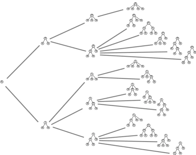
(2) P S N. N. P S N. N. N. P S. N. N. S P. N. N P S. N. N S P N. S P N. N. N. S P. P S N. S P N. N. N. N. P S. N. S P. N. P S N S P. P S. N P S. N N. N. S P. N. N. N P S S N. S P N. N. N. N N. N. N S. S N N. N. N. N P. N. N. N. N. S N. P N. N S. N. N N. S N. S P S N. N P N. N. N N. N. N P N S P. S P. N. N N. N. N. S N N. N. P S. N S P S P N. N. S P N. N. N. S. N. S P. N S. N. N. N. N P N S P N. N N. N. Figure 2: The family tree F4 .. parallel trees without repetition. Using similar method we can generate several planar structures [LN01, N02, N04]. In this paper we first extend the method for more general graphs. The rest of the paper is organized as follows. Section 2 gives some definitions. Section 3 introduces the family tree. Section 4 presents our algorithm. Finally Section 5 is a conclusion.. 2. Preliminaries. In this section we give some definitions. Let G be a connected graph with n vertices and m edges. A tree is a connected graph without cycles. A rooted tree is a tree with one vertex r chosen as its root. For each vertex v in a rooted tree, let U P (v) be the unique path from v to the root r. If U P (v) has exactly k edges then we say the depth of v is k, and write dep(v) = k. The parent of v 6= r is. its neighbor on U P (v), and ancestors of v 6= r are the vertices on U P (v) except v. The parent and the ancestors of r are not defined. We say that if v is the parent of u then u is a child of v, and if v is an ancestor of u then u is a descendant of v. A leaf is a vertex having no child. An ordered tree is a rooted tree with a left-to-right ordering specified for the children of each vertex. We denote by T (v) the ordered subtree of an ordered tree T consisting of a vertex v and all descendant of v preserving the left-to-right ordering for the children of each vertex. A graph G(s, t) is a series-parallel graph with terminals s and t, if (1) G consists of one edge connecting s and t, or (2) G is derived from two or more series-parallel graphs by one of the following two operations. • The series composition: Given k seriesparallel graphs G1 (s1 , t1 ), G2 (s2 , t2 ), . . .,. 2 −42−.

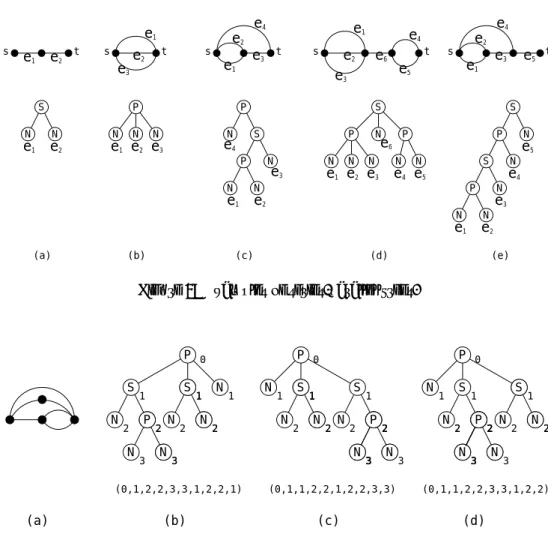
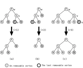
(3) Gk (sk , tk ), form a new graph G(s, t) by identifying s = s1 , t = tk , and ti = si+1 for 1 ≤ j ≤ k − 1. • The parallel composition: Given k seriesparallel graphs G1 (s1 , t1 ), G2 (s2 , t2 ), . . ., Gk (sk , tk ), form a new graph G(s, t) by identifying s = s1 = s2 = · · · = sk , and t = t1 = t2 = · · · = tk . Note that the ordering G1 (s1 , t1 ), G2 (s2 , t2 ), . . . , Gk (sk , tk ) matters for the series composition, while it does not matter for the parallel composition. The recursive definition of the series-parallel graph above naturally gives a tree T , called a series-parallel tree, for each series-parallel graph G(s, t). See some examples in Fig.3. Each leaf in T corresponds to an edge of G(s, t), and each non-leaf vertex in T corresponds to either series or parallel composition. We say that each vertex is normal, series, or parallel, respectively. We can observe that if the root vertex is series vertex, then every non-leaf vertex at even depth is also a series vertex, while every non-leaf vertex at odd depth is a parallel vertex. (The other case is similar.) Note that a series-parallel graph G may have many corresponding series-parallel trees, since we can choose any ordering for child vertices of each parallel vertex. We are going to assign a unique ordered tree for each series-parallel graph. We need some definitions here. Let T be an ordered tree with n vertices, and (v1 , v2 , . . . , vn ) be the vertices of T in preorder [A95]. Let dep(v) be the depth of v. Then the sequence L(T ) = (dep(v1 ), dep(v2 ), . . . , dep(vn )) is called the depth sequence. Let T1 and T2 be two ordered trees, and L(T1 ) = (a1 , a2 , . . . , ac ) and L(T2 ) = (b1 , b2 , . . . , bd ). Then we say that T1 is heavier than T2 , if ai = bi for each i = 1, 2, . . . , k−1 (possibly k = 1) and either ak > bk or c > k − 1 = d. Now we assign the heaviest ordered tree H for each series-parallel graph G. We call such the heaviest ordered tree H the canonical tree of G. Fig.4 (a) shows a series parallel graph G, and Fig.4 (b)– (d) show series-parallel ordered trees corresponding to G, with their depth sequences. The depth sequence of (b) is the heaviest, therefore neither (c) nor (d) is the canonical tree of G. Let Sm be the set of all canonical trees with at most m leaves. Note that each tree in Sm corresponds to each series-parallel graph having at most m edges. We have the following lemma.. Lemma 2.1 A series-parallel tree T is in Sm if and only if T has at most m leaves, and for every consecutive child vertices v1 and v2 of every parallel vertex, L(T (v1 )) ≥ L(T (v2 )) holds. Proof. By contradiction. Omitted. 2 We call the condition above “the left heavy condition”.. 3. The family tree. Assume m ≥ 2. Let T ∈ Sm , be a canonical tree. We say a vertex v in T is un-removable if v satisfies the following three conditions. (co1) v is normal, (co2) v is the rightmost vertex in its siblings, and (co3) v has exactly one sibling (except v). See some examples in Fig.5. A leaf v is removable if it is not un-removable. The last removable vertex of T in preorder is called the last removable vertex of T . Let u be the last removable vertex of T , and v the parent of u. Also let w be the parent of v if v is not the root of T . We define a new tree P (T ) as follows. We have the following two cases, depending on the number of child vertices of v. Case1: v has exactly two child vertices. Now v has two child leaves. We have the following two subcases. Case1–1: w has exactly two child vertices, and v is the right child of w. (r1) Then replace T (v) by one normal vertex. Note that the new vertex is un-removable. (See Fig.6(a).) Case1–2: Otherwise. Now we have two cases (1) w has exactly two vertices, and v is the left child of w, or (2) w has three or more child vertices, and v is the rightmost child of w. (r2) Then replace T (v) by one normal vertex. Note that the new vertex is removable. (See Fig.6(b).) Case2: v has three or more child vertices. (r3) Remove u. (see Fig.6(c).) Note that in all cases above, P (T ) has one less leaves than T . We say that P (T ) is the parent of T , and T is a child of P (T ). We have the following lemma. Lemma 3.1 If T is canonical then P (T ) is also canonical.. 3 −43−.

(4) e4. e1 s. e1. e2. t. s. t. e2. s. S. P. t. e3. e1. e3. s. e4. e2 e3. N. N. N. e2. e1 e2 e3. N. N. N. s. e3. e1. e5. e5. S S. P. P. N. N. e3 N. N. e1. e2. N. t. S. N. P. e6. e4. (b). e2 t. e6. P. e1. (a). e4. e1. e2. N. N. e5 N. e1 e2 e3. P N. S. N. e4 e5. e4 P. N. e3. (c). N. N. e1. e2. (d). (e). Figure 3: Examples of series-parallel trees.. P 0 S N. 2. N. S. 1. P. 3. N. 2. N. 2. 1. N. P 0 N. 1. N. N. 2. 2. S. 1. N. 2. N. 2. N. 3. (0,1,2,2,3,3,1,2,2,1). (a). S. 1. P 0 N. 1. P. 3. (0,1,1,2,2,1,2,2,3,3). (b). N. 2. N. 1. S. P. 2. N. 3. S. 1. 3. 2. N. N. 2. 1. N. 2. 3. (0,1,1,2,2,3,3,1,2,2). (c). (d). Figure 4: The depth sequences.. Proof. In P (T ), only subtrees rooted at vertices on the path between the root and the new vertex loose the “weight ”. So we need to check the left heavy condition for those subtrees. Since only trivial trees, consisting of one un-removable vertex, exist on the right of the subtrees above, the left heavy condition holds in P (T ). 2. Repeatedly applying above operations to any canonical tree T ∈ Sm , we have a sequence P (T ), P (P (T )), P (P (P (T ))), . . . of canonical trees, and the sequence eventually ends with the canonical tree having only one (normal) vertex. We denote the trivial canonical tree by T1 . See an example in Fig.7. By merging those sequences we have a tree Fm such that each vertex corresponds to a distinct canonical tree in Sm , each edge corresponds to. some relation between some T and P (T ). We call Fm the family tree of Sm . For instance F4 is shown in Fig.2.. 4. Algorithm. In this section we give an algorithm to construct Fm . We only consider the case the root of T is parallel. The other case is omitted since it is similar. Given a canonical tree T in Sm , if we have an algorithm to generate all child canonical trees of T , then in a recursive manner we can generate Fm , and which means we can generate all series-parallel graphs having at most m edges. How can we generate all child canonical trees of a given canonical tree ? As we will soon see we can do this by “reversing” the operations (r1)–(r3) in Section 3. Let T be a canonical tree in Sm , rk be the last removable vertex of T , and RP = (r0 , r1 , . . . , rk ). 4 −44−.

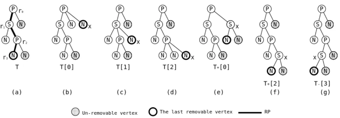
(5) S N. P N. N. P. N. N. S. N. S P. P N. N. N. N. S. N N. P N. P N. S. N. P N. N N. N N. The last removable vertex. Un-removable vertex. Figure 5: Examples of un-removable and removable vertex.. S w. S w. S w. P v S. P v N. N u N. N P N N. P v. N. N. N. (r3) N u. N. P N. P v. N. N u N. (r2). (r1). (r1). N u N The last removable vertex. Un-removable vertex. Figure 7: The removing sequence.. P w S N. P w S v. N. N u N. S v N N u N. (r1). N. S N. N. S v N. N. N. Un-removable vertex. (b). N u. P N. S N. (a). N. (r3). P N. N. (r2). P S. P w. N. S N. N. N. (c) The last removable vertex. Figure 6: Examples of operations (r1)–(r3).. be the path between the root r0 and rk . We construct three types of new trees T [i], T+ [i], T− , from T as follows. For i, 0 ≤ i ≤ k − 1, we define T [i] to be the canonical tree derived from T by (a1) adding a new vertex x as the rightmost child of ri . See some examples in Fig.8 (b)–(d). Note that the last removable vertex of T [i] is the new vertex x.. For i, 0 ≤ i ≤ k − 1, if ri has exactly two child vertices, and the right child vertex w of ri is normal, then we define T+ [i] to be the canonical tree derived from T by (a2) replacing w by either a series or parallel vertex x and add two normal child vertices to x. See Fig.8 (e) and (f). Note that the last removable vertex of T+ [i] is the left child of vertex x. By definition, rk−1 always has two normal child vertices. We define T− to be the canonical tree derived from T by (a3) replacing rk by either a series or parallel vertex x and add two normal child vertices to x. See Fig.8 (g). Note that the last removable vertex of T− is the left child vertex of x. We can observe that each operation (a1), (a2) and (a3) is the reverse of (r3), (r2) and (r1), respectively. Each derived tree has one more leaves than T . Define C(T ) = {T [0], T [1], . . . , T [k − 1]} ∪ {T+ [0], T+ [1], . . . , T+ [k − 1]} ∪ {T− }, those are candidates for child trees of T . We can observe that each child tree of T ∈ Sm is in C(T ), however, not all trees in C(T ) are child trees of T . For example, the tree T+ [2] in Fig.8(f) is not a child tree of T , since it is not a canonical tree, so T+ [2] 6∈ Sm . Thus we need to check whether each possible child. 5 −45−.

(6) P r0 r1 S. N. N. P r2. r3 N. (a). P. S. N. T. P N. N. N x. P N. N N. T[0]. (b). S. P N. P N. P. S N x. N. N. N. T[1]. S x N. N N. T[2]. (c). Un-removable vertex. S. P N. P. (d). N x. P N. N. N. P. S. N. N. N. T+[0]. (e). The last removable vertex. S. P N. N S x. N. T+[2] (f). N. N P. x S N. N N. T-[3] (g). RP. Figure 8: The possible child series-parallel trees.. tree is actually a child tree of T or not. We now have the following lemma. Lemma 4.1 Let T ∈ Sm , T 0 ∈ C(T ), rk be the last removable vertex of T 0 and RP = (r0 , r1 , . . . , rk ) be the path of T 0 between the root r0 and rk . Then T 0 is a child tree of T if and only if L(T 0 (si+1 )) ≥ L(T 0 (ri+1 )) holds for every parallel vertex ri , 0 ≤ i < k, on RP , where si+1 is the child of ri preceding ri+1 . Proof. Since T ∈ Sm , the left heavy condition has held in T . In T 0 some subtrees may be heavier than in T . So we must check if left heavy condition still holds or not. The claim checks all of these possible changes to destroy the left heavy condition. 2 If we generate each tree in C(T ) then check whether it is actually a child tree or not based on the lemma above, then we need much running time. However we can improve the running time as follows. We need some definition here. Let T be a canonical tree in Sm , rk be the last removable vertex of T . RP = (r0 , r1 , . . . , rk ) be the path of T between the root r0 and rk . Let Tr be the tree derived from T by removing all un-removable vertices. We say that T is active at depth i, 0 ≤ i ≤ k − 1, if (i) ri is a parallel vertex. (ii) ri has the child vertex si+1 preceding ri+1 . (iii) L(Tr (ri+1 )) is a prefix of L(Tr (si+1 )). Intuitively, if T is active at depth i, then we are copying subtree T (ri+1 ) from T (si+1 ). We say that the copy-depth of T is c if T is active at depth c but not active at each i ∈ {0, 1, . . . , c − 1}. Especially. if T is not active at any in {0, 1, . . . , k − 1}, then we define the copy depth of T is k. Now we are going to check each tree in C(T ) is actually a child tree of T or not. Let c be the copydepth of T . Assume that the root vertex of T is parallel vertex. (The other case is similar.) First we consider for T [i], 0 ≤ i < k.. Case T [i] We have the following four cases. Case 1: T has m leaves. Then T corresponds to a leaf in Fm . Hence T has no child tree. Case 2: Otherwise, c = k. In this case L(Tr (si+1 )) > L(Tr (ri+1 )) holds for each parallel vertex ri . Now T [0], T [1], . . . , T [k − 1] are all child trees of T . In each tree T [i], the last removable vertex is x. The copy-depth of T [i] is i for each even i, (that is a parallel vertex) and i + 1 for each odd i. For example, a tree T and some child trees are shown in Fig.9. In T [2], (i) r2 is parallel vertex, (ii) r2 has the child vertex y preceding r3 , (iii) L(Tr (r3 )) is a prefix of L(Tr (y)). Hence T [2] is active at depth 2 and the copy depth of T [2] is 2. In T [3], r3 is not parallel vertex. Hence r3 is not active and copy depth of T [3] is k = 4. Case 3: Otherwise, L(Tr (rc+1 )) = L(Tr (sc+1 )). (Intuitively the copy has completed.) In this case T [0], T [1], . . . , T [c] are child trees of T . The copy-depth of T [i] is i for each even i, and i+1 for each odd i. T [c + 1], T [c + 2], . . . , T [k − 1] are not child trees of T . Case 4: Otherwise. (Intuitively the copy has not completed yet.) Now L(Tr (sc+1 )) ≥ L(Tr (rc+1 )) holds. Let L(Tr (sc+1 )) = (dep(u1 ), dep(u2 ), . . ., dep(un0 ), . . ., dep(un00 )), L(Tr (rc+1 )) = (dep(v1 ), dep(v2 ),. 6 −46−.

(7) r0 P r1 S r2 P r3 S r4 N. r0 P N. r1 S. N. N. N. r2 P. N. S N. r0 P r1 S. N N. y. N. r2 P N. r3. r3 S. r0 P N. r1 S. N. r2 P. N. N N. r3 S N. r4 N. r4. T. T[2]. Un-removable vertex. The last removable vertex. T[3]. r0 P N. r1 S. N. N. P. N. S. r1 S P r2. N. N. r2 P. N. S. r3 N. N. N. N. N N S. y N. N. r3 N. r4. T RP. r0 P. T+[1]. Un-removable vertex. T+[2]. The last removable vertex. Figure 9: Illustrations for T [i].. Figure 10: Illustrations for T+ [i].. . . ., dep(vn0 )), and set d = dep(un0 +1 ). (Intuitively we are copying Tr (rc+1 ) from Tr (sc+1 ) and un0 +1 is the next vertex to be copied.) In this case T [0], T [1], . . . , T [d − 1] are child trees of T . For i = 0, 1, . . . , d − 2, The copy-depth of T [i] is i for each even i, and i + 1 for each odd i. The copydepth of T1 [d − 1] is remains at c. Next we consider for T+ [i], 0 ≤ i ≤ k − 1.. does not hold in T+ [k − 1]. Hence T+ [k − 1] is not a child tree of T . Case 3: Otherwise, L(Tr (rc+1 )) = L(Tr (sc+1 )). (Intuitively the copy has completed.) For each i, 0 ≤ i ≤ c − 1, such that ri has exactly two child vertices, and the right child vertex w of ri is normal, T+ [i] is a child tree of T . In T+ [i] the last removable vertex is the left child vertex of the new vertex replacing w. The copy-depth of T+ [i] is i for each even i, and i + 2 for each odd i. For i, i = c, ri has at least two child vertices ri+1 and si+1 preceding ri+1 . Hence ri does not has un-removable child vertex, and T+ [i] does not exist. Case 4: Otherwise. (Intuitively the copy has not completed yet.) Now L(Tr (sc+1 )) ≥ L(Tr (rc+1 )) holds. Let L(Tr (sc+1 )) = (dep(u1 ), dep(u2 ), . . . ,dep(un0 ), . . ., dep(un00 )), L(Tr (rc+1 )) = (dep(v1 ), dep(v2 ), . . ., dep(vn0 )), and set d = dep(un0 +1 ). (Intuitively we are copying Tr (rc+1 ) from Tr (sc+1 ) and un0 +1 is the next vertex to be copied.) For each i, 0 ≤ i ≤ d − 2, such that ri has exactly two child vertices, and the right child vertex w of ri is normal, T+ [i] is a child tree of T . For i ≥ d − 1, T+ [i] is not a child tree of T , since the left heavy condition does not hold at c. The copy-depth of T+ [i] is i for each even i, and i + 2 for each odd i. Next we consider for T− .. Case T+ [i] We have the following four cases. Case 1: T has m leaves. Then T corresponds to a leaf in Fm . Hence T has no child tree. Case 2: Otherwise, c = k. In this case L(Tr (si+1 )) > L(Tr (ri+1 )) holds for each parallel vertex ri . We have the following two subcases. Case 2-1: For each i, 0 ≤ i ≤ k − 2, such that ri has exactly two child vertex, and the right child vertex w of ri is normal, T+ [i] is a child tree of T . In T+ [i] the last removable vertex is the left child vertex of the new vertex replacing w. The copy-depth of T+ [i] is i for each even i, and i + 2 for each odd i. For example, see Fig.10. In T+ [2], L(Tr (r3 )) is a prefix of L(Tr (y)). Hence T+ [2] is active at depth 2 and the copy depth of T+ [2] is 2. In T+ [1], r2 has no child vertex preceding r3 . Hence r2 is not active, and the copy depth of T+ [1] is k = 3. Case 2-2: For i, i = k − 1. If rk−1 is series vertex, T+ [k − 1] is a child tree of T and the copy-depth of T+ [k − 1] is k + 1. If rk−1 is parallel vertex, rk−1 has exactly two child vertices and rk is the left child. (Otherwise rk is the right most child of rk−1 , and L(Tr (rk )) is a prefix of L(Tr (sk )), hence copy depth of T is k − 1. A contradiction.) In this case the left heavy condition. Case T− [i] We have the following four cases. Note that rk is the last removable vertex of T . Case 1: T has m leaves. Then T corresponds to a leaf in Fm . Hence T has no child tree. Case 2: Otherwise, c = k. In this case T− is a child tree of T , and the copy. 7 −47−. RP.

(8) depth of T− is k + 1. Case 3: Otherwise, L(Tr (rc+1 )) = L(Tr (sc+1 )). (Intuitively the copy has completed.) In this case T− is not a child tree of T . Case 4: Otherwise. (Intuitively the copy has not completed yet.) Now L(Tr (sc+1 )) > L(Tr (rc+1 )) holds. Let L(Tr (sc+1 )) = (dep(u1 ), dep(u2 ),. . . , dep(un0 ), . . . ,dep(un00 )), L(Tr (rc+1 )) =(dep(v1 ), dep(v2 ),. . . ,dep(vn0 )). (Intuitively we are copying Tr (cc+1 ) from Tr (sc+1 ) and un0 +1 is the next vertex to be copied.) We have the following two subcases. Case 4-1: dep(un0 ) + 1 = dep(un0 +1 ). In this case T− is a child tree of T , and the copy depth of T− remains at c. Case 4-2: Otherwise. T− is not a child tree of T . Based on the case analysis above we have the following theorem. Theorem 4.2 Given m, one can generate all series-parallel graphs with at most m edges without repetition in O(|Sm |) time.. 5. Conclusion. In this paper we have given a simple algorithm to generate all series-parallel graphs with at most m edges. Our algorithm first defines a family tree such that each vertex corresponds to each seriesparallel trees with at most m leaves, then outputs each graph without repetition by traversing the family tree.. 謝辞. [G93] L. A. Goldberg, Efficient Algorithms for Listing Combinatorial Structures, Cambridge University Press, New York, (1993). [KS98] D. L. Kreher and D. R. Stinson, CRC Press, Boca Raton, (1998). [LN01] Z. Li and S. Nakano, Efficient Generation of Plane Triangulations without Repetitions, Proc. ICALP2001, LNCS 2076, (2001), pp.433–443. [LR99] G. Li and F. Ruskey, The Advantage of Forward Thinking in Generating Rooted and Free Trees, Proc. 10th Annual ACMSIAM Symp. on Discrete Algorithms, (1999), pp.939–940. [M98] B. D. McKay, Isomorph-free Exhaustive Generation, J. of Algorithms, 26, (1998), pp.306-324. [N02] S. Nakano, Efficient Generation of Plane Trees, Information Processing Letters, 84, (2002), pp.167–172. [N04] S. Nakano, Efficient Generation of Triconnected Plane Triangulations, Computational Geometry Theory and Applications, Vol. 27(2), (2004), pp.109-122. [R78] R. C. Read, How to Avoid Isomorphism Search When Cataloguing Combinatorial Configurations, Annals of Discrete Mathematics, 2, (1978), pp.107–120. [W89] H. S. Wilf, Combinatorial Algorithms : An Update, SIAM, (1989). [W86] R. A. Wright, B. Richmond, A. Odlyzko and B. D. McKay, Constant Time Generation of Free Trees, SIAM J. Comput., 15, (1986), pp.540-548.. 本研究は国立情報学研究所の共同研究より支援を受けた.. References [A95] A. V. Aho and J. D. Ullman, Foundations of Computer Science, Computer Science Press, New York, (1995). [B80] T. Beyer and S. M. Hedetniemi, Constant Time Generation of Rooted Trees, SIAM J. Comput., 9, (1980), pp.706-712. 8 −48−.

(9)